library(patchwork)
library(mcmcplots)
library(ggmcmc)
library(tidybayes)
library(tmap)
tmap_mode("plot")
library(terra)
library(sf)
sf::sf_use_s2(FALSE)
library(tidyverse)
# options
options(scipen = 999)Leopardus wiedii Model Outputs
Model outputs for Leopardus wiedii.
- R Libraries
- Basemaps
equalareaCRS <-  '+proj=laea +lon_0=-73.125 +lat_0=0 +datum=WGS84 +units=m +no_defs'
latam <- st_read('data/latam.gpkg', layer = 'latam', quiet = T)
countries <- st_read('data/latam.gpkg', layer = 'countries', quiet = T)
latam_land <- st_read('data/latam.gpkg', layer = 'latam_land', quiet = T)
latam_raster <- rast('data/latam_raster.tif', lyrs='latam')
latam_countries <- rast('data/latam_raster.tif', lyrs='countries')

lwiedii_IUCN <- sf::st_read('big_data/lwiedii_IUCN.shp', quiet = T) %>% sf::st_transform(crs=equalareaCRS)- Species data and covariates
# Presence-absence data
lwiedii_expert_blob_time1 <- readRDS('data/species_POPA_data/lwiedii_expert_blob_time1.rds')
lwiedii_expert_blob_time2 <- readRDS('data/species_POPA_data/lwiedii_expert_blob_time2.rds')

PA_time1 <- readRDS('data/species_POPA_data/data_lwiedii_PA_time1.rds') %>%
  cbind(expert=lwiedii_expert_blob_time1) %>%
  filter(!is.na(env.bio_7) &!is.na(env.bio_10) & !is.na(env.npp) & !is.na(env.nontree) & !is.na(expert)) # remove NA's
PA_time2 <- readRDS('data/species_POPA_data/data_lwiedii_PA_time2.rds') %>%
  cbind(expert=lwiedii_expert_blob_time2) %>%
  filter(!is.na(env.bio_7) &!is.na(env.bio_10) & !is.na(env.npp) & !is.na(env.nontree) & !is.na(expert)) # remove NA's

# Presence-only data
lwiedii_expert_gridcell <- readRDS('data/species_POPA_data/lwiedii_expert_gridcell.rds')

PO_time1 <- readRDS('data/species_POPA_data/data_lwiedii_PO_time1.rds') %>%
  cbind(expert=lwiedii_expert_gridcell$dist_exprt) %>%
  filter(!is.na(env.bio_7) &!is.na(env.bio_10) & !is.na(env.npp) & !is.na(env.nontree) & !is.na(acce) & !is.na(count) & !is.na(expert)) # remove NA's
PO_time2  <- readRDS('data/species_POPA_data/data_lwiedii_PO_time2.rds')  %>%
  cbind(expert=lwiedii_expert_gridcell$dist_exprt) %>%
  filter(!is.na(env.bio_7) &!is.na(env.bio_10) & !is.na(env.npp) & !is.na(env.nontree) & !is.na(acce) & !is.na(count) & !is.na(expert)) # remove NA's

PA_time1_time2 <- rbind(PA_time1 %>% mutate(time=1), PA_time2 %>% mutate(time=2))
PO_time1_time2 <- rbind(PO_time1 %>% mutate(time=1), PO_time2 %>% mutate(time=2)) - Read model
fitted.model <- readRDS('D:/Flo/JAGS_models/lwiedii_model.rds') # deleted after model output

# as.mcmc.rjags converts an rjags Object to an mcmc or mcmc.list Object.
fitted.model.mcmc <- mcmcplots::as.mcmc.rjags(fitted.model)
Model diagnostics
The fitted.model is an object of class rjags.
Code
# labels for the linear predictor `b`
L.fitted.model.b <- plab("b",
                         list(Covariate = c('Intercept',
                                            'env.bio_7',
                                            'env.bio_10',
                                            'env.npp',
                                            'env.nontree',
                                            'expert',
                                            sprintf('spline%i', 1:18)))) # changes with n.spl

# tibble object for the linear predictor `b` extracted from the rjags fitted model
fitted.model.ggs.b <- ggmcmc::ggs(fitted.model.mcmc,
                                  par_labels = L.fitted.model.b,
                                  family="^b\\[")

# diagnostics
ggmcmc::ggmcmc(fitted.model.ggs.b, file="docs/lwiedii_model_diagnostics.pdf", param_page=3)
Plotting histogramsPlotting density plotsPlotting traceplotsPlotting running meansPlotting comparison of partial and full chainPlotting autocorrelation plotsPlotting crosscorrelation plotPlotting Potential Scale Reduction FactorsPlotting shrinkage of Potential Scale Reduction FactorsPlotting Number of effective independent drawsPlotting Geweke DiagnosticPlotting caterpillar plotTime taken to generate the report: 31 seconds.Traceplot
Code
ggs_traceplot(fitted.model.ggs.b)
Rhat
Code
ggs_Rhat(fitted.model.ggs.b)
Probability of occurrence of Leopardus wiedii
For each period: time1 and time2, and their difference (time2-time1)
Code
P.pred <- fitted.model$BUGSoutput$mean$P.pred
preds <- data.frame(PO_time1_time2, P.pred)
preds1 <- preds[preds$time == 1,]
preds2 <- preds[preds$time == 2,]

rast <- latam_raster
rast[] <- NA
rast1 <- rast2 <- terra::rast(rast)

rast1[preds1$pixel] <- preds1$P.pred
rast2[preds2$pixel] <- preds2$P.pred

rast1 <- rast1 %>% terra::mask(., vect(latam_land))
rast2 <- rast2 %>% terra::mask(., vect(latam_land))
names(rast1) <- 'time1'
names(rast2) <- 'time2'

# Map of the of the probability of occurrence in the first period (time1: 2000-2013)
time1MAP <- tm_graticules(alpha = 0.3) +
    tm_shape(rast1) +
    tm_raster(palette = 'Oranges', midpoint = NA, style= "cont")  +
    tm_shape(countries) +
    tm_borders(col='grey60', alpha = 0.4) +
    tm_layout(legend.outside = T, frame.lwd = 0.3, scale=1.2, legend.outside.size = 0.1)

# Map of the of the probability of occurrence in the second period (time2: 2014-2021)
time2MAP <- tm_graticules(alpha = 0.3) +
    tm_shape(rast2) +
    tm_raster(palette = 'Purples', midpoint = NA, style= "cont")  +
    tm_shape(countries) +
    tm_borders(col='grey60', alpha = 0.4) +
    tm_layout(legend.outside = T, frame.lwd = 0.3, scale=1.2, legend.outside.size = 0.1)

# Map of the of the change in the probability of occurrence (time2 - time1)
diffMAP <- tm_graticules(alpha = 0.3) +
    tm_shape(rast2 - rast1) +
    tm_raster(palette = 'PiYG', midpoint = 0, style= "cont", ) +
    tm_shape(countries) +
    tm_borders(col='grey60', alpha = 0.4) +
    tm_layout(legend.outside = T, frame.lwd = 0.3, scale=1.2, legend.outside.size = 0.1)

time1MAP
Code
time2MAP
Code
diffMAP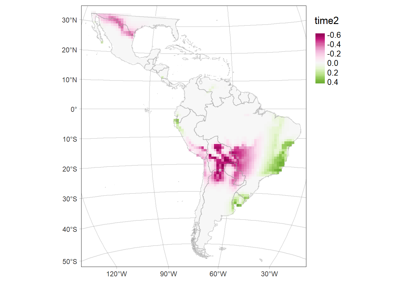
Code
tmap::tmap_save(tm = time1MAP, filename = 'docs/figs/time1MAP_SR_lwiedii.svg', device = svglite::svglite)
tmap::tmap_save(tm = time2MAP, filename = 'docs/figs/time2MAP_SR_lwiedii.svg', device = svglite::svglite)
Standard deviation (SD) of the probability of occurrence of Leopardus wiedii
Code
P.pred.sd <- fitted.model$BUGSoutput$sd$P.pred
preds.sd <- data.frame(PO_time1_time2, P.pred.sd)

preds1.sd <- preds.sd[preds.sd$time == 1,]
preds2.sd <- preds.sd[preds.sd$time == 2,]

rast.sd <- terra::rast(latam_raster)
rast.sd[] <- NA
rast1.sd <- rast2.sd <- terra::rast(rast.sd)

rast1.sd[preds1.sd$pixel] <- preds1.sd$P.pred.sd
rast2.sd[preds2.sd$pixel] <- preds2.sd$P.pred.sd

rast1.sd <- rast1.sd %>% terra::mask(., vect(latam_land))
rast2.sd <- rast2.sd %>% terra::mask(., vect(latam_land))
names(rast1.sd) <- 'time1.sd'
names(rast2.sd) <- 'time2.sd'

# Map of the SD of the probability of occurrence of the area time1
time1MAP.sd <- tm_graticules(alpha = 0.3) +
    tm_shape(rast1.sd) +
    tm_raster(palette = 'Oranges', midpoint = NA, style= "cont")  +
    tm_shape(countries) +
    tm_borders(alpha = 0.3) +
    tm_layout(legend.outside = T, frame.lwd = 0.3, scale=1.2, legend.outside.size = 0.1)

# Map of the SD of the probability of occurrence of the area time2
time2MAP.sd <-  tm_graticules(alpha = 0.3) +
    tm_shape(rast2.sd) +
    tm_raster(palette = 'Purples', midpoint = NA, style= "cont")  +
    tm_shape(countries) +
    tm_borders(alpha = 0.3) +
    tm_layout(legend.outside = T, frame.lwd = 0.3, scale=1.2, legend.outside.size = 0.1)

time1MAP.sd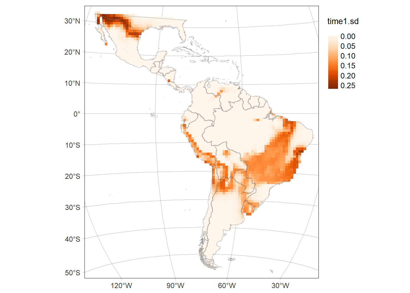
Code
time2MAP.sd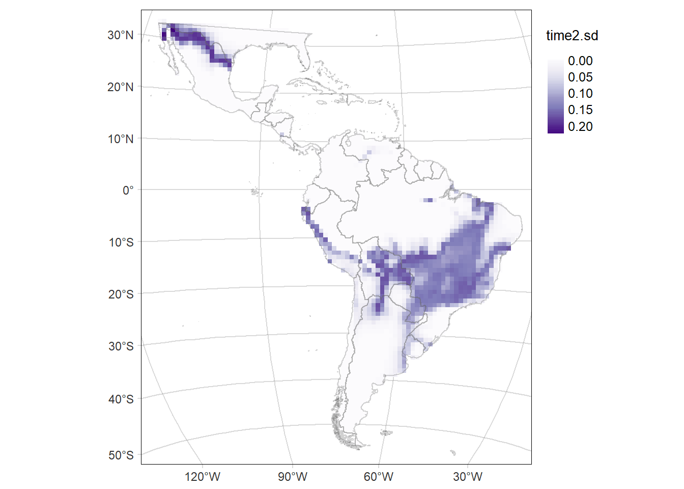
Bivariate map
Map of the difference including the Standard deviation (SD) of the probability of occurrence as the transparency of the layer.
Code
library(cols4all)
library(pals)
library(classInt)
library(stars)

bivcol = function(pal, nx = 3, ny = 3){
  tit = substitute(pal)
  if (is.function(pal))
    pal = pal()
  ncol = length(pal)
  if (missing(nx))
    nx = sqrt(ncol)
  if (missing(ny))
    ny = nx
  image(matrix(1:ncol, nrow = ny), axes = FALSE, col = pal, asp = 1)
  mtext(tit)
}

lwiedii.pal.pu_gn_bivd <- c4a("pu_gn_bivd", n=3, m=5)
lwiedii.pal <- c(t(apply(lwiedii.pal.pu_gn_bivd, 2, rev)))

###

pred.P.sd <- fitted.model$BUGSoutput$sd$delta.Grid
preds.sd <- data.frame(PO_time1_time2, pred.P.sd=rep(pred.P.sd, 2))

rast.sd <- terra::rast(latam_raster)
rast.sd[] <- NA
rast.sd <- terra::rast(rast.sd)

rast.sd[preds.sd$pixel] <- preds.sd$pred.P.sd
rast.sd <- rast.sd %>% terra::mask(., vect(latam_land))
names(rast.sd) <- c('diff')

# Map of the SD of the probability of occurrence of the area time2
delta.GridMAP.sd <-  tm_graticules(alpha = 0.3) +
    tm_shape(rast.sd) +
    tm_raster(palette = 'Greys', midpoint = NA, style= "cont")  +
    tm_shape(countries) +
    tm_borders(alpha = 0.3) +
    tm_layout(legend.outside = T, frame.lwd = 0.3, scale=1.2, legend.outside.size = 0.1)

delta.GridMAP.sd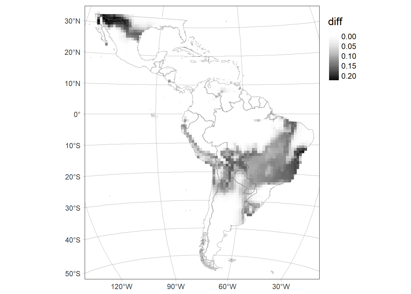
Code
rast.stars <- c(stars::st_as_stars(rast2-rast1), stars::st_as_stars(rast.sd))
names(rast.stars) <- c('diff', 'sd')

par(mfrow=c(2,2))
hist(rast1)
hist(rast2)
hist(rast.stars['diff'])
hist(rast.stars['sd'])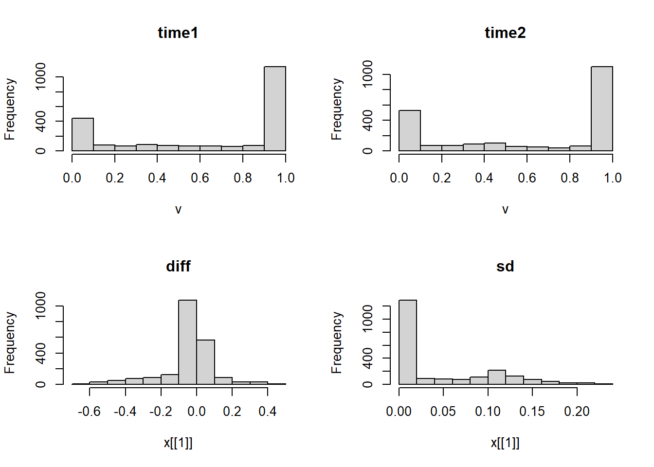
Code
par(mfrow=c(1,1))

add_new_var = function(x, var1, var2, nbins1, nbins2, style1, style2,fixedBreaks1, fixedBreaks2){
  class1 = suppressWarnings(findCols(classIntervals(c(x[[var1]]),
                                                    n = nbins1,
                                                    style = style1,
                                                    fixedBreaks1=fixedBreaks1)))

  class2 = suppressWarnings(findCols(classIntervals(c(x[[var2]]),
                                                    n = nbins2,
                                                    style = style2,
                                                    fixedBreaks=fixedBreaks2)))

  x$new_var = class1 + nbins1 * (class2 - 1)
  return(x)
}

rast.bivariate = add_new_var(rast.stars,
                             var1 = "diff",
                             var2 = "sd",
                             nbins1 = 3,
                             nbins2 = 5,
                             style1 = "fixed",
                             fixedBreaks1=c(-1,-0.05, 0.05, 1),
                             style2 = "fixed",
                             fixedBreaks2=c(0, 0.05, 0.1, 0.15, 0.2, 0.3))


# See missing classes and update palette
all_classes <- seq(1,15,1)
rast_classes <- as_tibble(rast.bivariate['new_var']) %>%
    distinct(new_var) %>% filter(!is.na(new_var)) %>% pull()
absent_classes <- all_classes[!(all_classes %in% rast_classes)]

if (length(absent_classes)==0){
  lwiedii.new.pal <- lwiedii.pal
} else lwiedii.new.pal <- lwiedii.pal[-c(absent_classes)]

# Map of the of the change in the probability of occurrence (time2 - time1)
# according to the mean SD of the probability of occurrence  (mean(time2.sd, time1.sd))

diffMAP.SD <- tm_graticules(alpha = 0.3) +
  tm_shape(rast.bivariate) +
  tm_raster("new_var", style= "cat", palette = lwiedii.new.pal) +
  tm_shape(countries) +
  tm_borders(col='grey60', alpha = 0.4) +
  tm_layout(legend.outside = T, frame.lwd = 0.3, scale=1.2, legend.outside.size = 0.1)

diffMAP.SD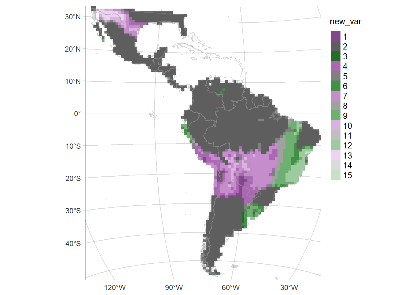
Code
tmap::tmap_save(tm = diffMAP.SD, filename = 'docs/figs/diffMAP_SD_lwiedii.svg', device = svglite::svglite)Countries thinning
Code
countryLevels <- cats(latam_countries)[[1]] #%>% mutate(value=value+1)
rasterLevels <- levels(as.factor(PO_time1_time2$country))
countries_latam <- countryLevels %>% filter(value %in% rasterLevels) %>%
  mutate(numLevel=1:length(rasterLevels)) %>% rename(country=countries)

fitted.model.ggs.alpha <- ggmcmc::ggs(fitted.model.mcmc, family="^alpha")
ci.alpha <- ci(fitted.model.ggs.alpha)

country_acce <- bind_rows(ci.alpha[length(rasterLevels)+1,],
          tibble(countries_latam, ci.alpha[1:length(rasterLevels),])) %>%
  dplyr::select(-c(value, numLevel))

#accessibility range for predictions
accessValues <- seq (0,0.5,by=0.01)

#get common steepness
commonSlope <- country_acce$median[country_acce$Parameter=="alpha1"]

#write function to get predictions for a given country
getPreds <- function(country){
  #get country intercept
  countryIntercept = country_acce$median[country_acce$country==country & !is.na(country_acce$country)]
  #return all info
  data.frame(country = country,
             access = accessValues,
             preds= countryIntercept * exp(((-1 * commonSlope)*accessValues)))
}

allPredictions <- country_acce %>%
                  filter(!is.na(country)) %>%
                  filter(country %in% countries$iso_a2) %>%
                  pull(country) %>%
                  map_dfr(getPreds)

allPredictions <- left_join(as_tibble(allPredictions),
                            countries %>% select(country=iso_a2, name_en) %>%
                              st_drop_geometry(), by='country') %>%
  filter(country!='VG' & country!= 'TT' & country!= 'FK' & country!='AW')

# just for exploration - easier to see which county is doing which
acce_country <- ggplot(allPredictions)+
    geom_line(aes(x = access, y  = preds, colour = name_en), show.legend = F) +
    viridis::scale_color_viridis(option = 'turbo', discrete=TRUE) +
    theme_bw() +
    facet_wrap(~name_en, ncol = 5) +
    ylab("Probability of retention") + xlab("Accessibility")

acce_country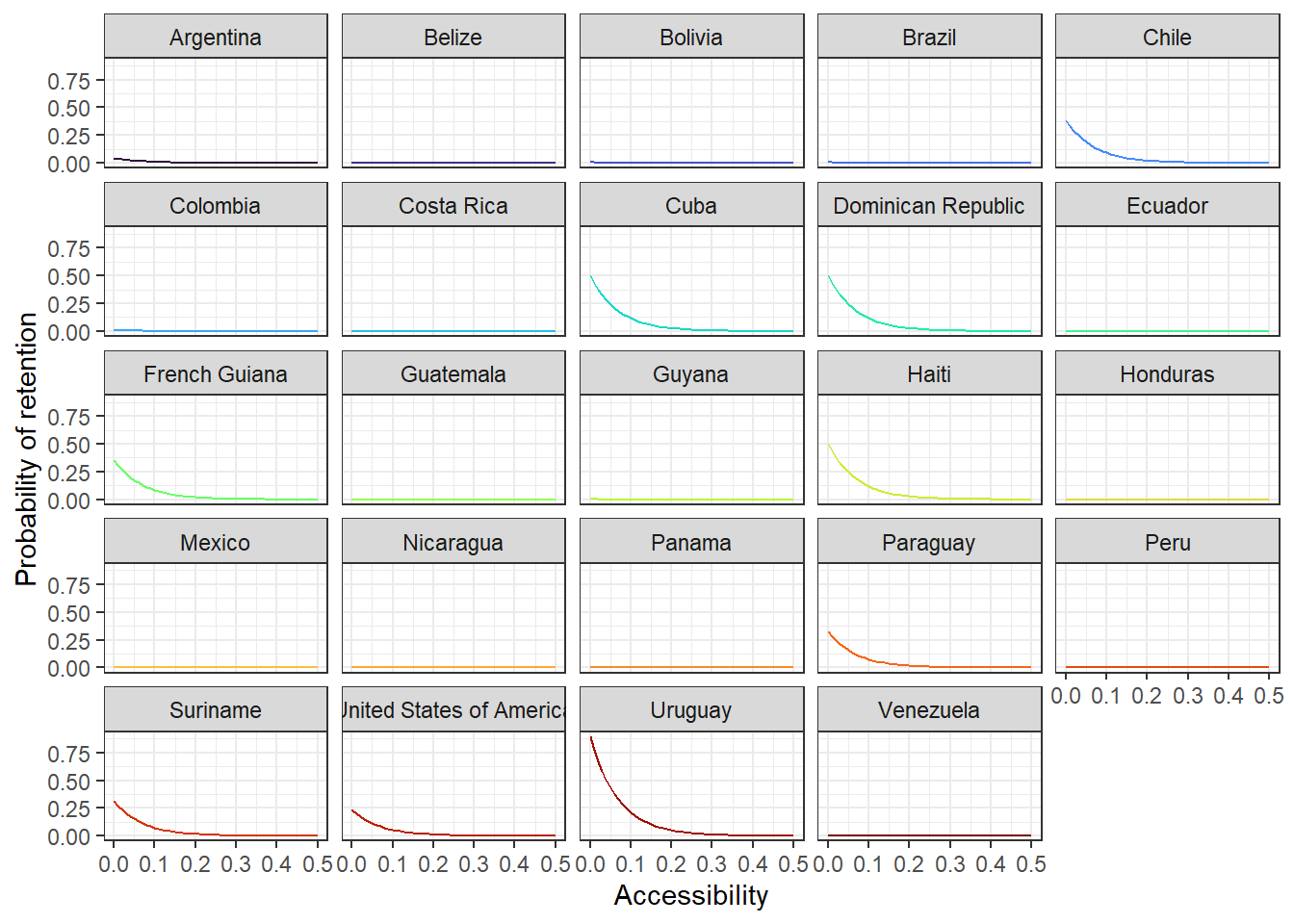
Code
# all countries
acce_allcountries <- ggplot(allPredictions) +
  geom_line(aes(x = access, y  = preds, colour = name_en), show.legend = F)+
  viridis::scale_color_viridis(option = 'turbo', discrete=TRUE) +
  theme_bw() +
  ylab("Probability of retention") + xlab("Accessibility")

acce_allcountries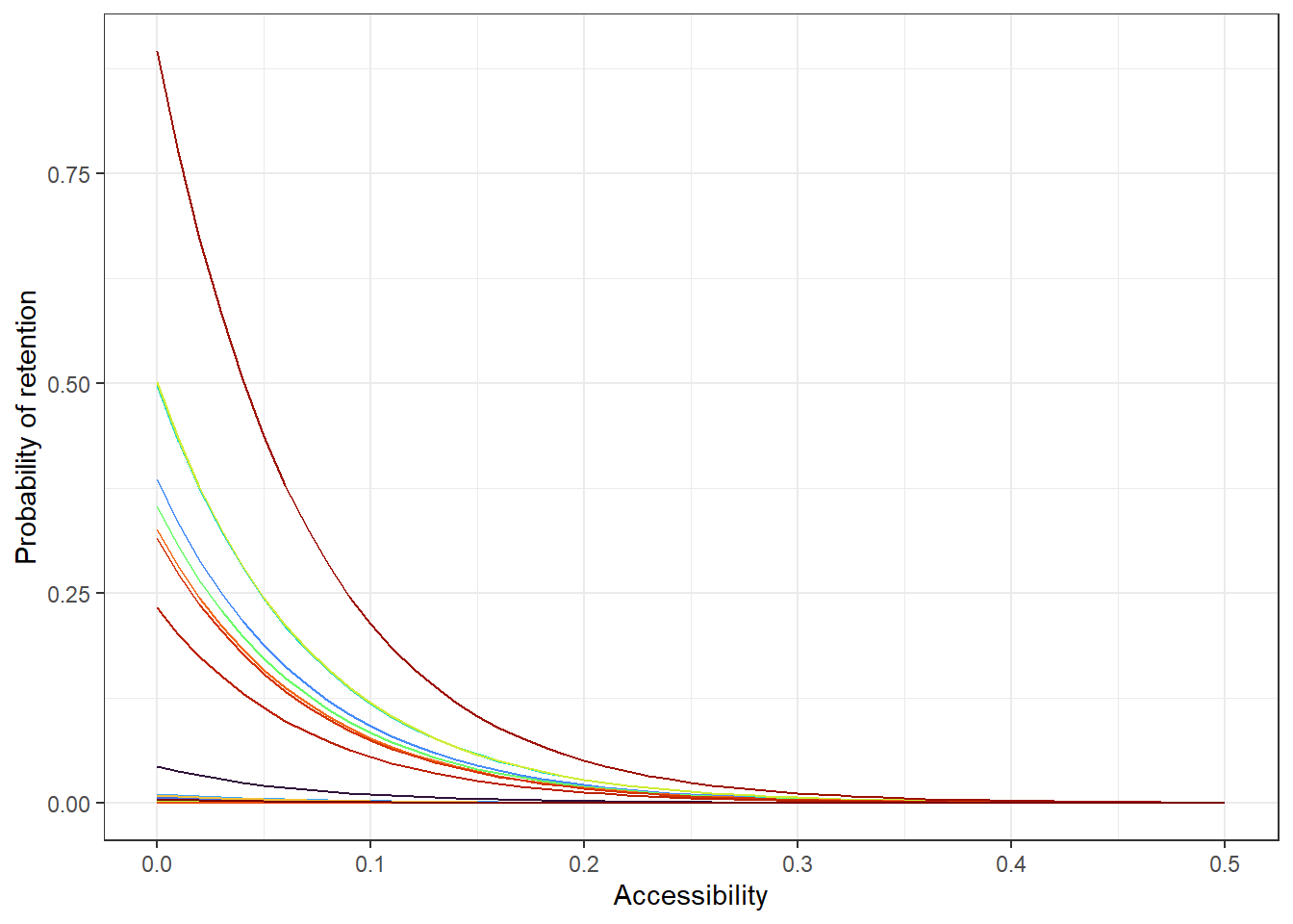
Effect of the environmental covariates on the intensity of the point process
Code
caterpiller.params <- fitted.model.ggs.b %>%
  filter(grepl('env', Parameter)) %>%
  mutate(Parameter=as.factor(ifelse(Parameter=='env.bio_7', 'bio_7',
                                    ifelse(Parameter=='env.nontree', 'nontree',
                                           ifelse(Parameter=='env.npp', 'npp',
                                                  ifelse(Parameter=='env.bio_10', 'bio_10', Parameter)))))) %>%
  ggs_caterpillar(line=0) +
  theme_light() +
  labs(y='', x='posterior densities')

caterpiller.params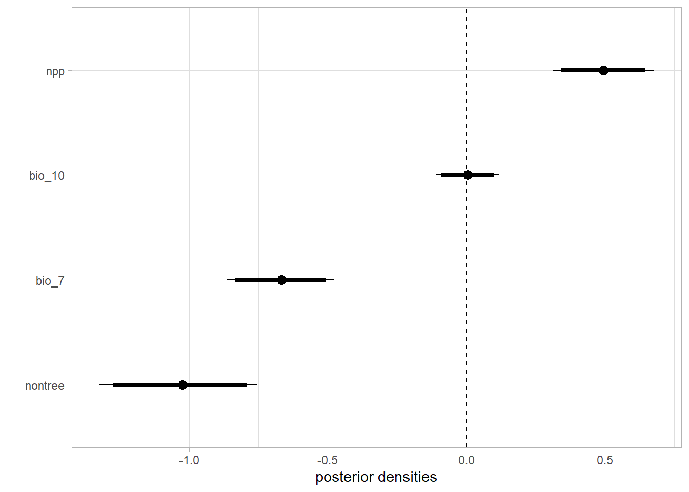
Boxplot of posterior densities of the predicted area in both time periods
Code
fitted.model.ggs.A <- ggmcmc::ggs(fitted.model.mcmc,  family="^A")

# CI
ggmcmc::ci(fitted.model.ggs.A)
# A tibble: 2 x 6
Parameter low Low median High high
<fct> <dbl> <dbl> <dbl> <dbl> <dbl>
1 A.time1 1316. 1334. 1427. 1516. 1532.
2 A.time2 1240. 1258. 1350. 1444. 1462.Code
fitted.model$BUGSoutput$summary['A.time2',] mean sd 2.5% 25% 50% 75%
1350.593856 56.350451 1239.679519 1312.310314 1350.034978 1388.904974
97.5% Rhat n.eff
1461.514468 1.001216 7300.000000 Code
# fitted.model$BUGSoutput$mean$A.time2
fitted.model$BUGSoutput$summary['A.time1',]
mean sd 2.5% 25% 50% 75%
1425.936498 55.460947 1316.197260 1388.581784 1426.617502 1463.995143
97.5% Rhat n.eff
1532.185813 1.001215 7400.000000 Code
# fitted.model$BUGSoutput$mean$A.time1

# boxplot
range.boxplot <- ggs_caterpillar(fitted.model.ggs.A, horizontal=FALSE, ) + theme_light(base_size = 14) +
    labs(y='', x='Area (number of 100x100 km grid-cells)')

range.boxplot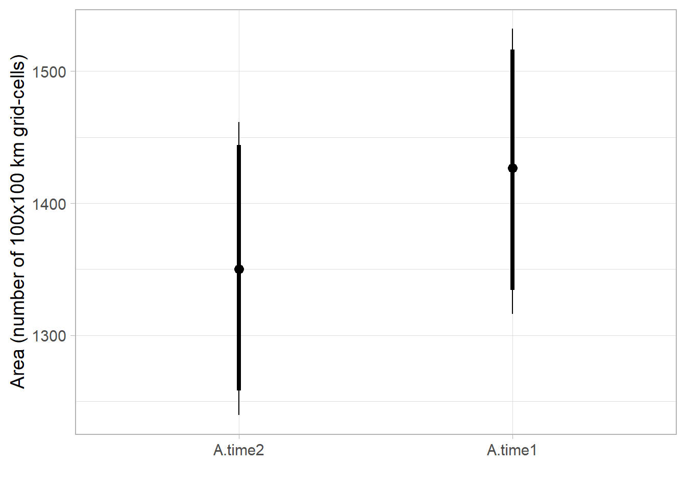
Code
# CI
range.ci <- ggmcmc::ci(fitted.model.ggs.A) %>%
    mutate(Parameter = fct_rev(Parameter)) %>%
    ggplot(aes(x = Parameter, y = median, ymin = low, ymax = high)) +
    geom_boxplot(orientation = 'y', size=1) +
    stat_summary(fun=mean, geom="point",
                 shape=19, size=4, show.legend=FALSE) +
    theme_light(base_size = 14) +
    labs(x='', y='Area (number of 100x100 km grid-cells)')

range.ci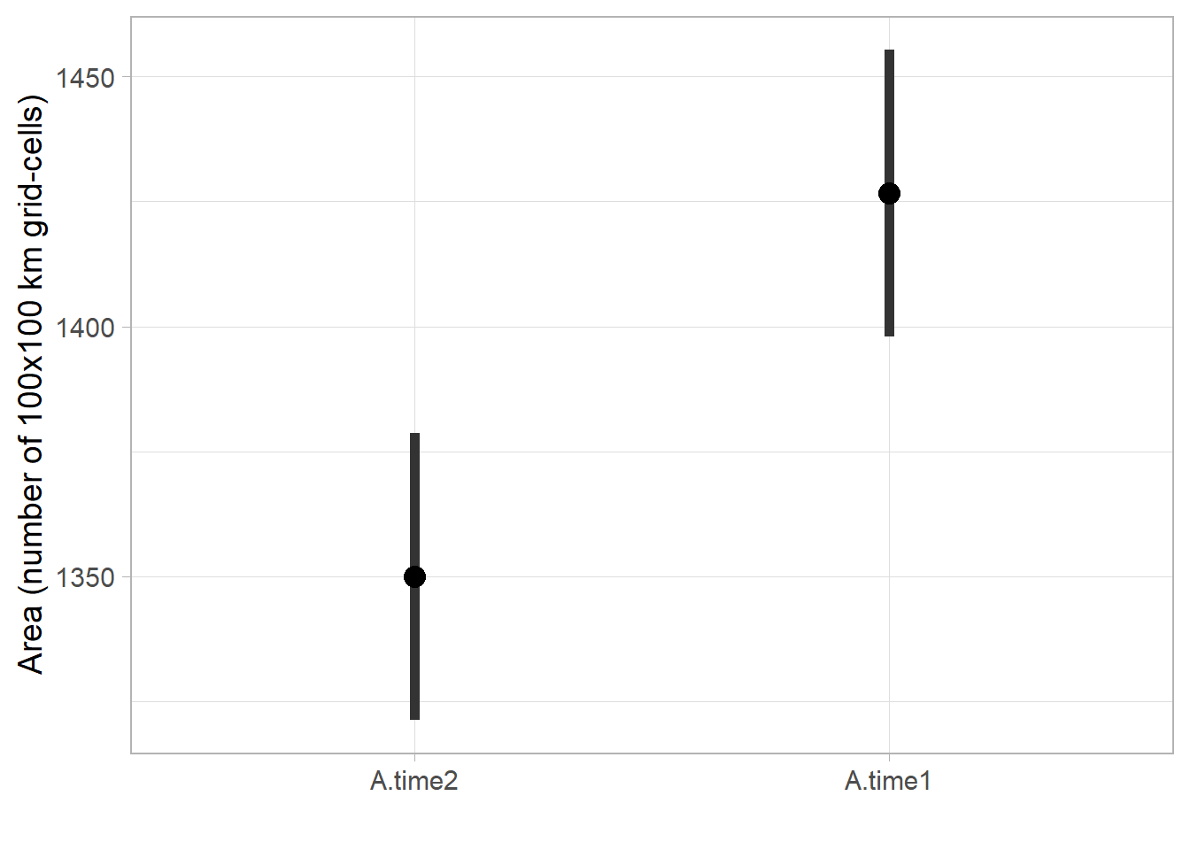
posterior distribution of range change (Area).
Code
fitted.model.ggs.delta.A <- ggmcmc::ggs(fitted.model.mcmc,  family="^delta.A")

# CI
ggmcmc::ci(fitted.model.ggs.delta.A)
# A tibble: 1 x 6
Parameter low Low median High high
<fct> <dbl> <dbl> <dbl> <dbl> <dbl>
1 delta.A -138. -129. -75.6 -21.1 -11.0Code
fitted.model$BUGSoutput$summary['delta.A',] mean sd 2.5% 25% 50% 75%
-75.342642 33.080618 -138.232857 -98.802694 -75.614213 -52.266133
97.5% Rhat n.eff
-11.032945 1.000966 27000.000000 Code
#densitiy
delta.A.plot <- fitted.model.ggs.delta.A %>% group_by(Iteration) %>%
    summarise(area=median(value)) %>%
    ggplot(aes(area)) +
    geom_density(col='grey30', fill='black', alpha = 0.3, size=1) +
    #scale_y_continuous(breaks=c(0,0.0025,0.005, 0.0075, 0.01, 0.0125)) +
    geom_abline(intercept = 0, slope=1, linetype=2, size=1) +
    # vertical lines at 95% CI
    stat_boxplot(geom = "vline", aes(xintercept = ..xmax..), size=0.5, col='red') +
    stat_boxplot(geom = "vline", aes(xintercept = ..xmiddle..), size=0.5, col='red') +
    stat_boxplot(geom = "vline", aes(xintercept = ..xmin..), size=0.5, col='red') +
    theme_light(base_size = 14, base_line_size = 0.2) +
    labs(y='Probability density', x=expression(Delta*'Area'))

delta.A.plot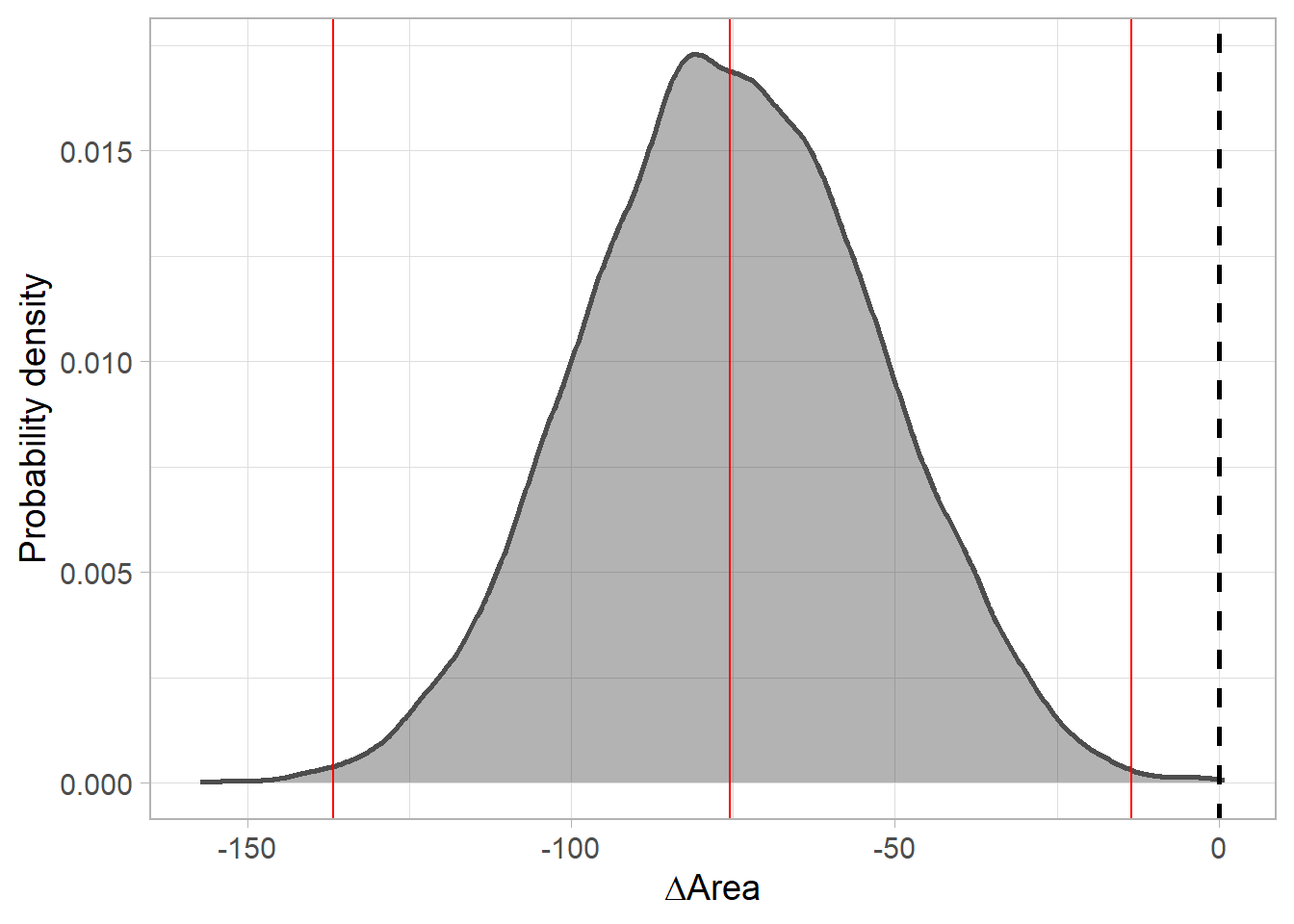
Code
ggsave(delta.A.plot, filename='docs/figs/delta_A_lwiedii.svg', device = 'svg', dpi=300)posterior predictive checks
PO
Expected vs observed
Code
counts <- PO_time1_time2$count
counts.new <- fitted.model$BUGSoutput$mean$y.PO.new
lambda <- fitted.model$BUGSoutput$mean$lambda
pred.PO <- data.frame(counts, counts.new, lambda)

# fitted.model$BUGSoutput$summary['fit.PO',]
# fitted.model$BUGSoutput$summary['fit.PO.new',]

pp.PO <- ggplot(pred.PO, aes(x=counts, y=lambda), fill=NA) +
    geom_point(size=3, shape=21)  +
    xlim(c(0, 100)) +
    ylim(c(0, 50)) +
    labs(x='observed', y=expression(lambda), title='Presence-only') +
    geom_abline(col='red') +
    theme_bw()

pp.PO.log10 <- ggplot(pred.PO, aes(x=counts, y=lambda), fill=NA) +
    geom_point(size=3, shape=21)  +
    scale_x_log10(limits=c(0.01, 100)) +
    scale_y_log10(limits=c(0.01, 100)) +
    coord_fixed(ratio=1) +
    labs(x='observed (log scale)', y=expression(lambda*'(log scale)'), title='log10 scale') +
    geom_abline(col='red') +
    theme_bw()

pp.PO | pp.PO.log10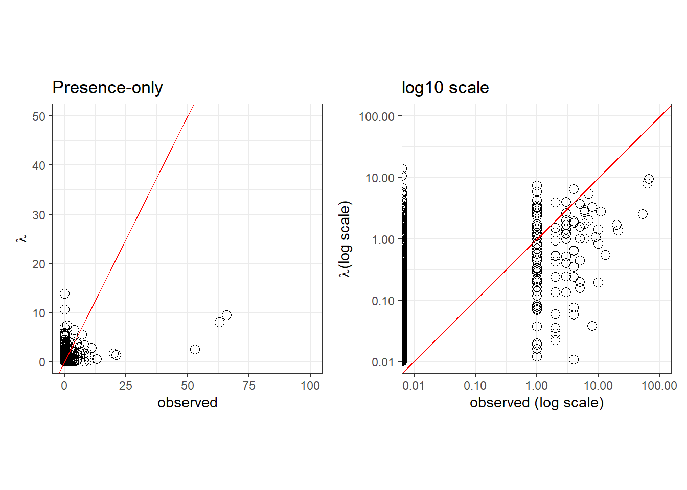
Residual Diagnostics
Code
library(DHARMa)

simulations <- fitted.model$BUGSoutput$sims.list$y.PO.new
pred <- apply(fitted.model$BUGSoutput$sims.list$lambda, 2, median)
#dim(simulations)

sim <- createDHARMa(simulatedResponse = t(simulations),
                    observedResponse = PO_time1_time2$count,
                    fittedPredictedResponse = pred,
                    integerResponse = T)

plotSimulatedResiduals(sim)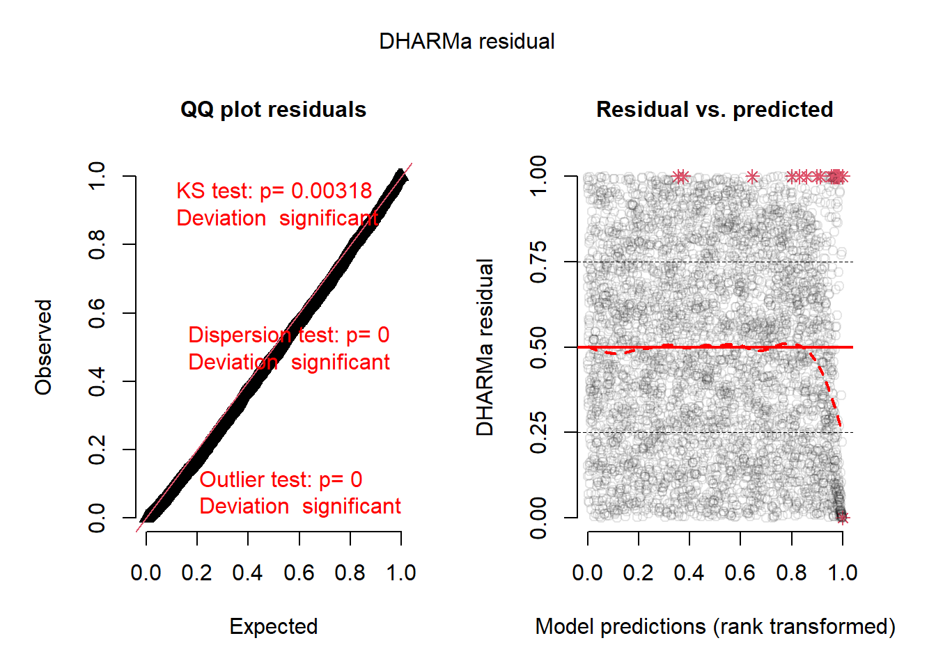
Grid-level change
Code
range_change <- as_tibble(rast2[PO_time2$pixel] - rast1[PO_time2$pixel]) %>% rename(range=time2)
numRecord_change <- as_tibble(PO_time2$count - PO_time1$count) %>% rename(numRecord=value)

grid.level.change <- bind_cols(range_change, numRecord_change) %>%
    mutate(nonzero=ifelse(numRecord==0, '0', '>=1')) %>%
    ggplot() +
    geom_point(aes(y=range, x=numRecord, col=nonzero), size=1) +
    geom_vline(xintercept=0, linetype=2, size=0.5) +
    geom_hline(yintercept=0, linetype=2, size=0.5) +
    labs(y = expression('Predicted grid-level range change (Ppred'['time2']*'-Ppred'['time1']*')'),
         x= expression('Grid-level range change in number of records (Nrecords'['time2']*'-Nrecords'['time1']*')'),
         col = 'Number of records\nper grid cell') +
    theme_bw(base_size = 14)

grid.level.change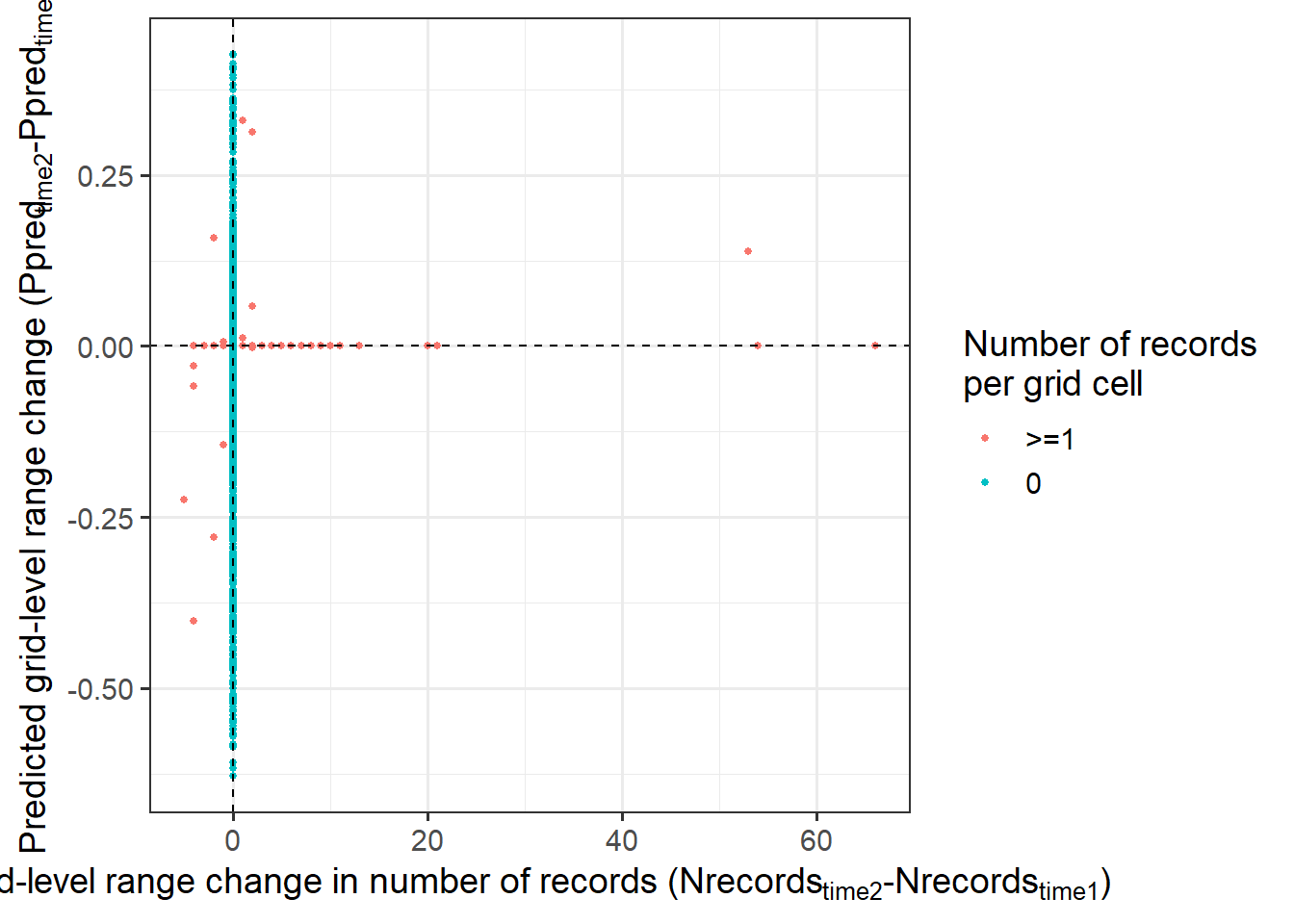
PA
Tjur R2
Code
presabs <- PA_time1_time2$presabs
psi <- fitted.model$BUGSoutput$mean$psi
pred.PA <- data.frame(presabs, psi)

r2_tjur <- round(fitted.model$BUGSoutput$mean$r2_tjur, 3)
fitted.model$BUGSoutput$summary['r2_tjur',]
mean sd 2.5% 25% 50%
0.376984352 0.005899612 0.365651126 0.372994580 0.376947812
75% 97.5% Rhat n.eff
0.380895833 0.388707255 1.002546052 1300.000000000 Code
pp.PA <- ggplot(pred.PA, aes(x=presabs, y=psi, col=presabs)) +
    geom_jitter(height = 0, width = .05, size=1)  +
    scale_x_continuous(breaks=seq(0,1,0.25)) + scale_colour_binned() +
    labs(x='observed', y=expression(psi), title='Presence-absence') +
    stat_summary(
        fun = mean,
        geom = "errorbar",
        aes(ymax = ..y.., ymin = ..y..),
        width = 0.2, size=2) +
    theme_bw() + theme(legend.position = 'none')+
    annotate(geom="text", x=0.5, y=0.5,
             label=paste('Tjur R-squared = ', r2_tjur))

pp.PA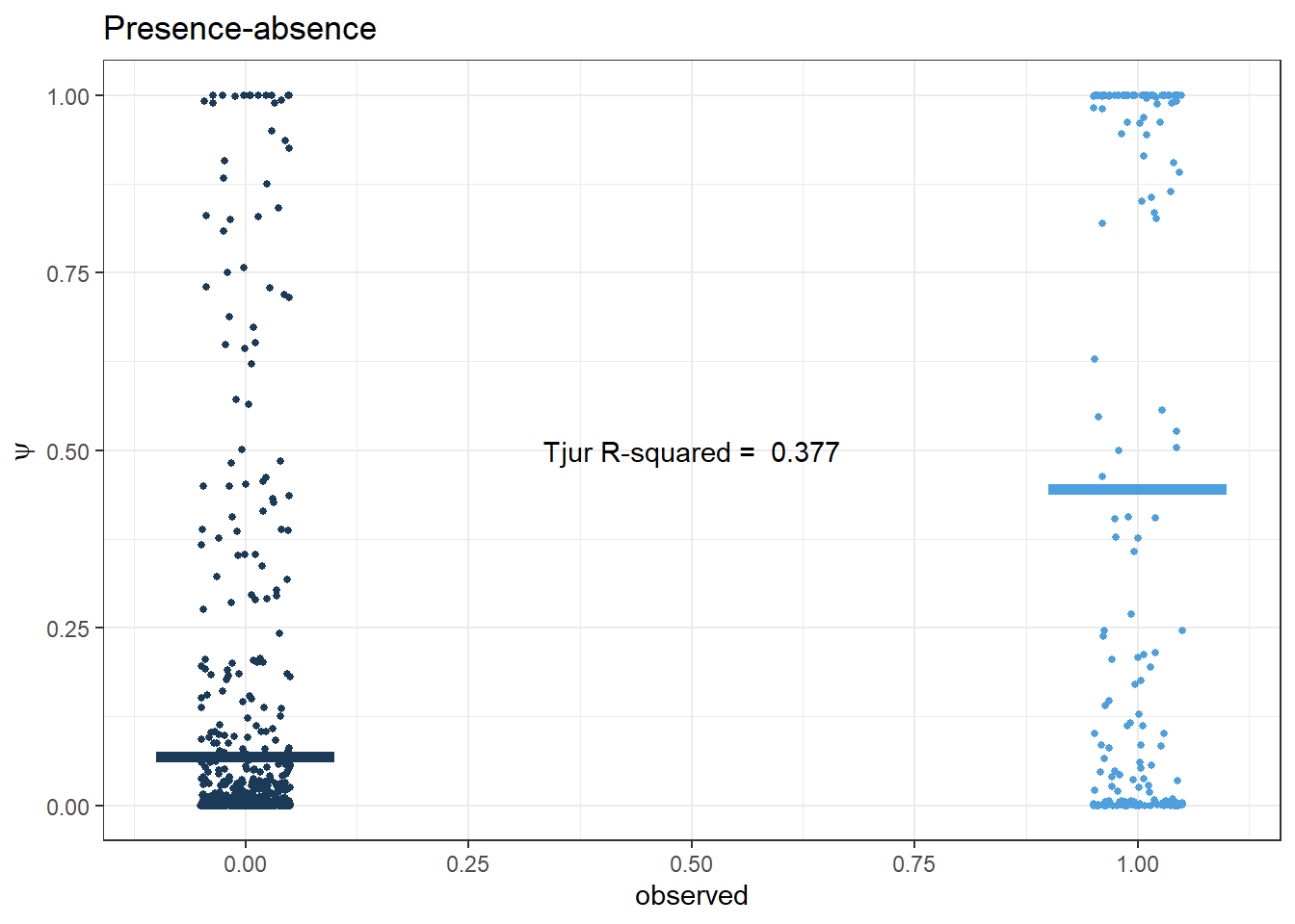
AUC
Code
auc.sens.fpr <- bind_cols(sens=fitted.model$BUGSoutput$mean$sens,
                          fpr=fitted.model$BUGSoutput$mean$fpr)

auc.value <- round(fitted.model$BUGSoutput$mean$auc, 3)

ggplot(auc.sens.fpr, aes(fpr, sens)) +
  geom_line() + geom_point() +
  labs(x='1 - Specificity', y='Sensitivity') +
  annotate(geom="text", x=0.5, y=0.5,
           label=paste('AUC = ', auc.value)) +
  theme_bw()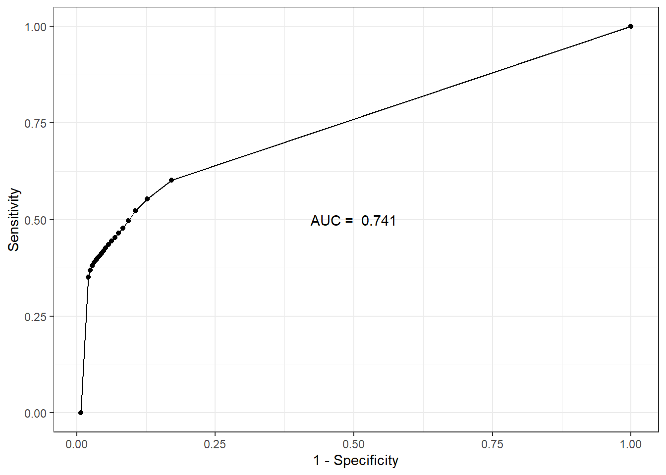
Code
fitted.model$BUGSoutput$summary['auc',] mean sd 2.5% 25% 50%
0.740900796 0.005243076 0.730636031 0.737413344 0.740859141
75% 97.5% Rhat n.eff
0.744419217 0.751279100 1.000998645 27000.000000000