library(patchwork)
library(mcmcplots)
library(ggmcmc)
library(tidybayes)
library(tmap)
tmap_mode("plot")
library(terra)
library(sf)
sf::sf_use_s2(FALSE)
library(tidyverse)
# options
options(scipen = 999)Leopardus pardalis Model Outputs
Model outputs for Leopardus pardalis.
- R Libraries
- Basemaps
equalareaCRS <-  '+proj=laea +lon_0=-73.125 +lat_0=0 +datum=WGS84 +units=m +no_defs'
latam <- st_read('data/latam.gpkg', layer = 'latam', quiet = T)
countries <- st_read('data/latam.gpkg', layer = 'countries', quiet = T)
latam_land <- st_read('data/latam.gpkg', layer = 'latam_land', quiet = T)
latam_raster <- rast('data/latam_raster.tif', lyrs='latam')
latam_countries <- rast('data/latam_raster.tif', lyrs='countries')

lpardalis_IUCN <- sf::st_read('big_data/lpardalis_IUCN.shp', quiet = T) %>% sf::st_transform(crs=equalareaCRS)- Species data and covariates
# Presence-absence data
lpardalis_expert_blob_time1 <- readRDS('data/species_POPA_data/lpardalis_expert_blob_time1.rds')
lpardalis_expert_blob_time2 <- readRDS('data/species_POPA_data/lpardalis_expert_blob_time2.rds')

PA_time1 <- readRDS('data/species_POPA_data/data_lpardalis_PA_time1.rds') %>%
  cbind(expert=lpardalis_expert_blob_time1) %>%
  filter(!is.na(env.bio_10) &!is.na(env.bio_17) & !is.na(env.npp) & !is.na(env.tree) & !is.na(expert)) # remove NA's
PA_time2 <- readRDS('data/species_POPA_data/data_lpardalis_PA_time2.rds') %>%
  cbind(expert=lpardalis_expert_blob_time2) %>%
  filter(!is.na(env.bio_10) &!is.na(env.bio_17) & !is.na(env.npp) & !is.na(env.tree) & !is.na(expert)) # remove NA's

# Presence-only data
lpardalis_expert_gridcell <- readRDS('data/species_POPA_data/lpardalis_expert_gridcell.rds')

PO_time1 <- readRDS('data/species_POPA_data/data_lpardalis_PO_time1.rds') %>%
  cbind(expert=lpardalis_expert_gridcell$dist_exprt) %>%
  filter(!is.na(env.bio_10) &!is.na(env.bio_17) & !is.na(env.npp) & !is.na(env.tree) & !is.na(acce) & !is.na(count) & !is.na(expert)) # remove NA's
PO_time2  <- readRDS('data/species_POPA_data/data_lpardalis_PO_time2.rds')  %>%
  cbind(expert=lpardalis_expert_gridcell$dist_exprt) %>%
  filter(!is.na(env.bio_10) &!is.na(env.bio_17) & !is.na(env.npp) & !is.na(env.tree) & !is.na(acce) & !is.na(count) & !is.na(expert)) # remove NA's

PA_time1_time2 <- rbind(PA_time1 %>% mutate(time=1), PA_time2 %>% mutate(time=2))
PO_time1_time2 <- rbind(PO_time1 %>% mutate(time=1), PO_time2 %>% mutate(time=2)) - Read model
fitted.model <- readRDS('D:/Flo/JAGS_models/lpardalis_model.rds') # deleted after model output

# as.mcmc.rjags converts an rjags Object to an mcmc or mcmc.list Object.
fitted.model.mcmc <- mcmcplots::as.mcmc.rjags(fitted.model)
Model diagnostics
The fitted.model is an object of class rjags.
Code
# labels for the linear predictor `b`
L.fitted.model.b <- plab("b",
                         list(Covariate = c('Intercept',
                                            'env.bio_10',
                                            'env.bio_17',
                                            'env.tree',
                                            'env.npp',
                                            'expert',
                                            sprintf('spline%i', 1:12)))) # changes with n.spl

# tibble object for the linear predictor `b` extracted from the rjags fitted model
fitted.model.ggs.b <- ggmcmc::ggs(fitted.model.mcmc,
                                  par_labels = L.fitted.model.b,
                                  family="^b\\[")

# diagnostics
ggmcmc::ggmcmc(fitted.model.ggs.b, file="docs/lpardalis_model_diagnostics.pdf", param_page=3)
Plotting histogramsPlotting density plotsPlotting traceplotsPlotting running meansPlotting comparison of partial and full chainPlotting autocorrelation plotsPlotting crosscorrelation plotPlotting Potential Scale Reduction FactorsPlotting shrinkage of Potential Scale Reduction FactorsPlotting Number of effective independent drawsPlotting Geweke DiagnosticPlotting caterpillar plotTime taken to generate the report: 35 seconds.Traceplot
Code
ggs_traceplot(fitted.model.ggs.b)
Rhat
Code
ggs_Rhat(fitted.model.ggs.b)
Probability of occurrence of Leopardus pardalis
For each period: time1 and time2, and their difference (time2-time1)
Code
P.pred <- fitted.model$BUGSoutput$mean$P.pred
preds <- data.frame(PO_time1_time2, P.pred)
preds1 <- preds[preds$time == 1,]
preds2 <- preds[preds$time == 2,]

rast <- latam_raster
rast[] <- NA
rast1 <- rast2 <- terra::rast(rast)

rast1[preds1$pixel] <- preds1$P.pred
rast2[preds2$pixel] <- preds2$P.pred

rast1 <- rast1 %>% terra::mask(., vect(latam_land))
rast2 <- rast2 %>% terra::mask(., vect(latam_land))
names(rast1) <- 'time1'
names(rast2) <- 'time2'

# Map of the of the probability of occurrence in the first period (time1: 2000-2013)
time1MAP <- tm_graticules(alpha = 0.3) +
    tm_shape(rast1) +
    tm_raster(palette = 'Oranges', midpoint = NA, style= "cont")  +
    tm_shape(countries) +
    tm_borders(col='grey60', alpha = 0.4) +
    tm_layout(legend.outside = T, frame.lwd = 0.3, scale=1.2, legend.outside.size = 0.1)

# Map of the of the probability of occurrence in the second period (time2: 2014-2021)
time2MAP <- tm_graticules(alpha = 0.3) +
    tm_shape(rast2) +
    tm_raster(palette = 'Purples', midpoint = NA, style= "cont")  +
    tm_shape(countries) +
    tm_borders(col='grey60', alpha = 0.4) +
    tm_layout(legend.outside = T, frame.lwd = 0.3, scale=1.2, legend.outside.size = 0.1)

# Map of the of the change in the probability of occurrence (time2 - time1)
diffMAP <- tm_graticules(alpha = 0.3) +
    tm_shape(rast2 - rast1) +
    tm_raster(palette = 'PiYG', midpoint = 0, style= "cont", ) +
    tm_shape(countries) +
    tm_borders(col='grey60', alpha = 0.4) +
    tm_layout(legend.outside = T, frame.lwd = 0.3, scale=1.2, legend.outside.size = 0.1)

time1MAP
Code
time2MAP
Code
diffMAP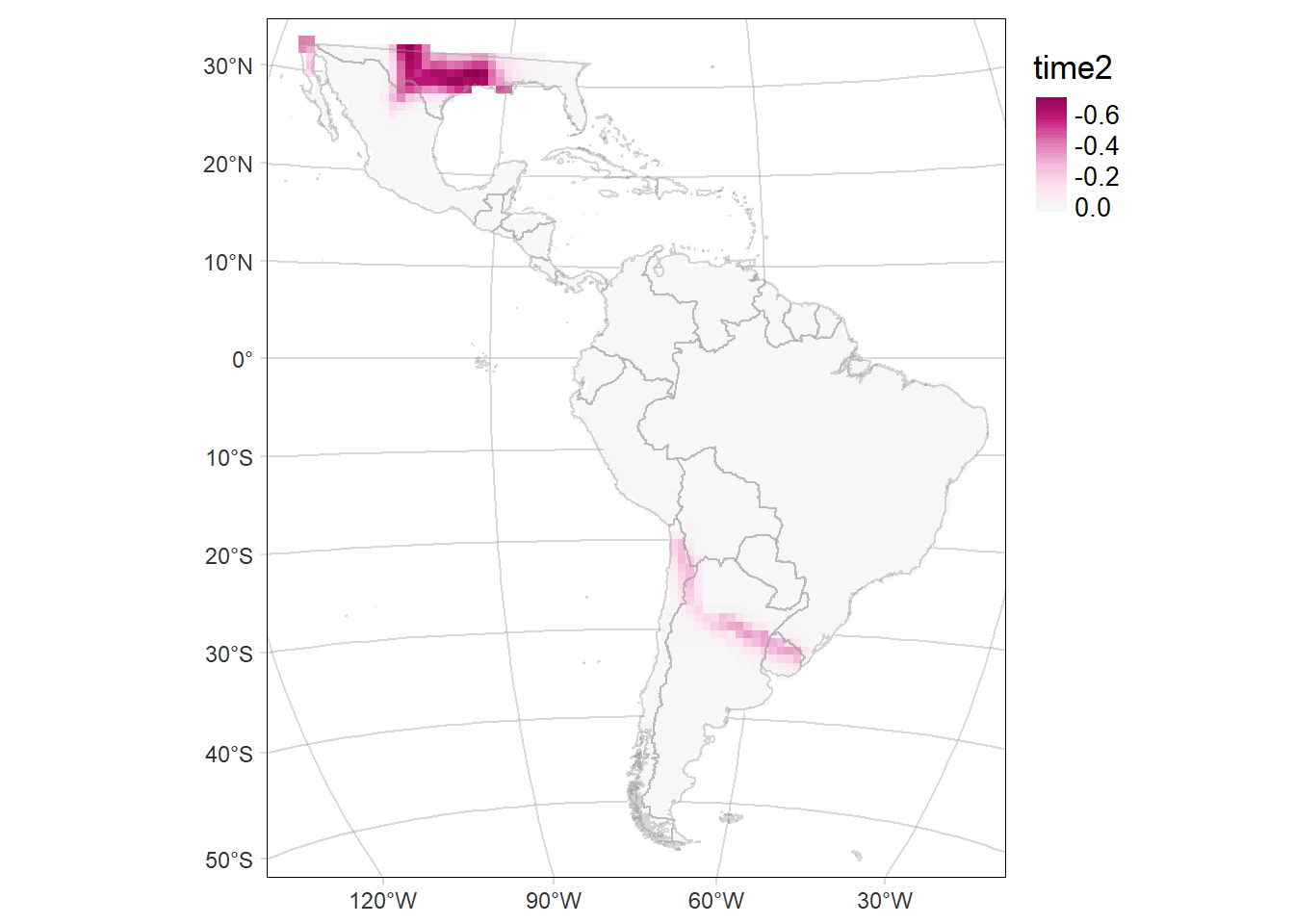
Code
tmap::tmap_save(tm = time1MAP, filename = 'docs/figs/time1MAP_SR_lpardalis.svg', device = svglite::svglite)
tmap::tmap_save(tm = time2MAP, filename = 'docs/figs/time2MAP_SR_lpardalis.svg', device = svglite::svglite)
Standard deviation (SD) of the probability of occurrence of Leopardus pardalis
Code
P.pred.sd <- fitted.model$BUGSoutput$sd$P.pred
preds.sd <- data.frame(PO_time1_time2, P.pred.sd)

preds1.sd <- preds.sd[preds.sd$time == 1,]
preds2.sd <- preds.sd[preds.sd$time == 2,]

rast.sd <- terra::rast(latam_raster)
rast.sd[] <- NA
rast1.sd <- rast2.sd <- terra::rast(rast.sd)

rast1.sd[preds1.sd$pixel] <- preds1.sd$P.pred.sd
rast2.sd[preds2.sd$pixel] <- preds2.sd$P.pred.sd

rast1.sd <- rast1.sd %>% terra::mask(., vect(latam_land))
rast2.sd <- rast2.sd %>% terra::mask(., vect(latam_land))
names(rast1.sd) <- 'time1.sd'
names(rast2.sd) <- 'time2.sd'

# Map of the SD of the probability of occurrence of the area time1
time1MAP.sd <- tm_graticules(alpha = 0.3) +
    tm_shape(rast1.sd) +
    tm_raster(palette = 'Oranges', midpoint = NA, style= "cont")  +
    tm_shape(countries) +
    tm_borders(alpha = 0.3) +
    tm_layout(legend.outside = T, frame.lwd = 0.3, scale=1.2, legend.outside.size = 0.1)

# Map of the SD of the probability of occurrence of the area time2
time2MAP.sd <-  tm_graticules(alpha = 0.3) +
    tm_shape(rast2.sd) +
    tm_raster(palette = 'Purples', midpoint = NA, style= "cont")  +
    tm_shape(countries) +
    tm_borders(alpha = 0.3) +
    tm_layout(legend.outside = T, frame.lwd = 0.3, scale=1.2, legend.outside.size = 0.1)

time1MAP.sd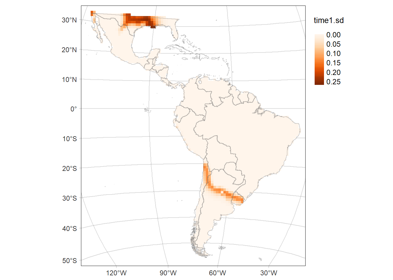
Code
time2MAP.sd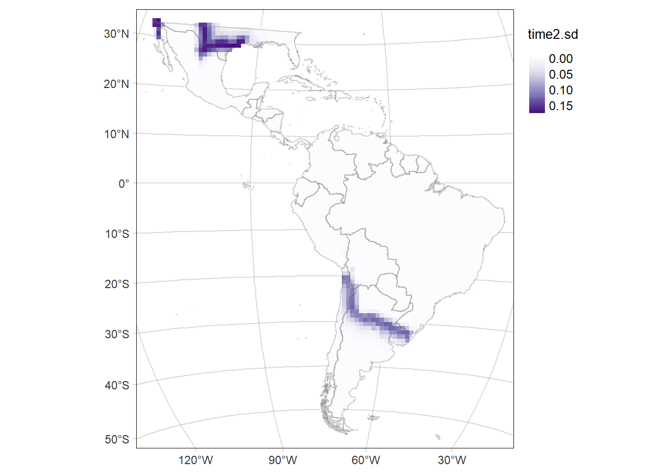
Bivariate map
Map of the difference including the Standard deviation (SD) of the probability of occurrence as the transparency of the layer.
Code
library(cols4all)
library(pals)
library(classInt)
library(stars)

bivcol = function(pal, nx = 3, ny = 3){
  tit = substitute(pal)
  if (is.function(pal))
    pal = pal()
  ncol = length(pal)
  if (missing(nx))
    nx = sqrt(ncol)
  if (missing(ny))
    ny = nx
  image(matrix(1:ncol, nrow = ny), axes = FALSE, col = pal, asp = 1)
  mtext(tit)
}

lpardalis.pal.pu_gn_bivd <- c4a("pu_gn_bivd", n=3, m=5)
lpardalis.pal <- c(t(apply(lpardalis.pal.pu_gn_bivd, 2, rev)))

###

pred.P.sd <- fitted.model$BUGSoutput$sd$delta.Grid
preds.sd <- data.frame(PO_time1_time2, pred.P.sd=rep(pred.P.sd, 2))

rast.sd <- terra::rast(latam_raster)
rast.sd[] <- NA
rast.sd <- terra::rast(rast.sd)

rast.sd[preds.sd$pixel] <- preds.sd$pred.P.sd
rast.sd <- rast.sd %>% terra::mask(., vect(latam_land))
names(rast.sd) <- c('diff')

# Map of the SD of the probability of occurrence of the area time2
delta.GridMAP.sd <-  tm_graticules(alpha = 0.3) +
    tm_shape(rast.sd) +
    tm_raster(palette = 'Greys', midpoint = NA, style= "cont")  +
    tm_shape(countries) +
    tm_borders(alpha = 0.3) +
    tm_layout(legend.outside = T, frame.lwd = 0.3, scale=1.2, legend.outside.size = 0.1)

delta.GridMAP.sd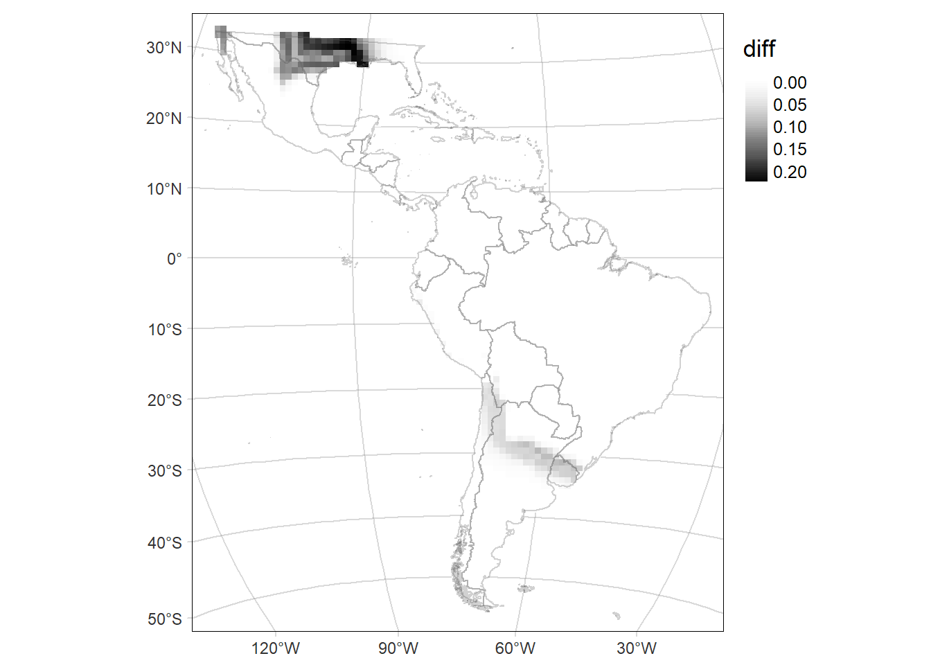
Code
rast.stars <- c(stars::st_as_stars(rast2-rast1), stars::st_as_stars(rast.sd))
names(rast.stars) <- c('diff', 'sd')

par(mfrow=c(2,2))
hist(rast1)
hist(rast2)
hist(rast.stars['diff'])
hist(rast.stars['sd'])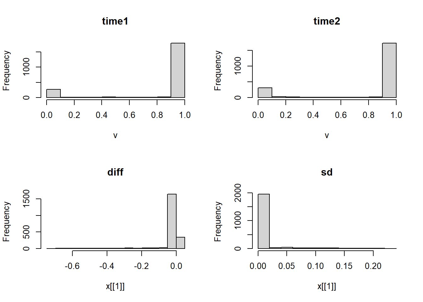
Code
par(mfrow=c(1,1))

add_new_var = function(x, var1, var2, nbins1, nbins2, style1, style2,fixedBreaks1, fixedBreaks2){
  class1 = suppressWarnings(findCols(classIntervals(c(x[[var1]]),
                                                    n = nbins1,
                                                    style = style1,
                                                    fixedBreaks1=fixedBreaks1)))

  class2 = suppressWarnings(findCols(classIntervals(c(x[[var2]]),
                                                    n = nbins2,
                                                    style = style2,
                                                    fixedBreaks=fixedBreaks2)))

  x$new_var = class1 + nbins1 * (class2 - 1)
  return(x)
}

rast.bivariate = add_new_var(rast.stars,
                             var1 = "diff",
                             var2 = "sd",
                             nbins1 = 3,
                             nbins2 = 5,
                             style1 = "fixed",
                             fixedBreaks1=c(-1,-0.05, 0.05, 1),
                             style2 = "fixed",
                             fixedBreaks2=c(0, 0.05, 0.1, 0.15, 0.2, 0.3))


# See missing classes and update palette
all_classes <- seq(1,15,1)
rast_classes <- as_tibble(rast.bivariate['new_var']) %>%
    distinct(new_var) %>% filter(!is.na(new_var)) %>% pull()
absent_classes <- all_classes[!(all_classes %in% rast_classes)]

if (length(absent_classes)==0){
  lpardalis.new.pal <- lpardalis.pal
} else lpardalis.new.pal <- lpardalis.pal[-c(absent_classes)]

# Map of the of the change in the probability of occurrence (time2 - time1)
# according to the mean SD of the probability of occurrence  (mean(time2.sd, time1.sd))

diffMAP.SD <- tm_graticules(alpha = 0.3) +
  tm_shape(rast.bivariate) +
  tm_raster("new_var", style= "cat", palette = lpardalis.new.pal) +
  tm_shape(countries) +
  tm_borders(col='grey60', alpha = 0.4) +
  tm_layout(legend.outside = T, frame.lwd = 0.3, scale=1.2, legend.outside.size = 0.1)

diffMAP.SD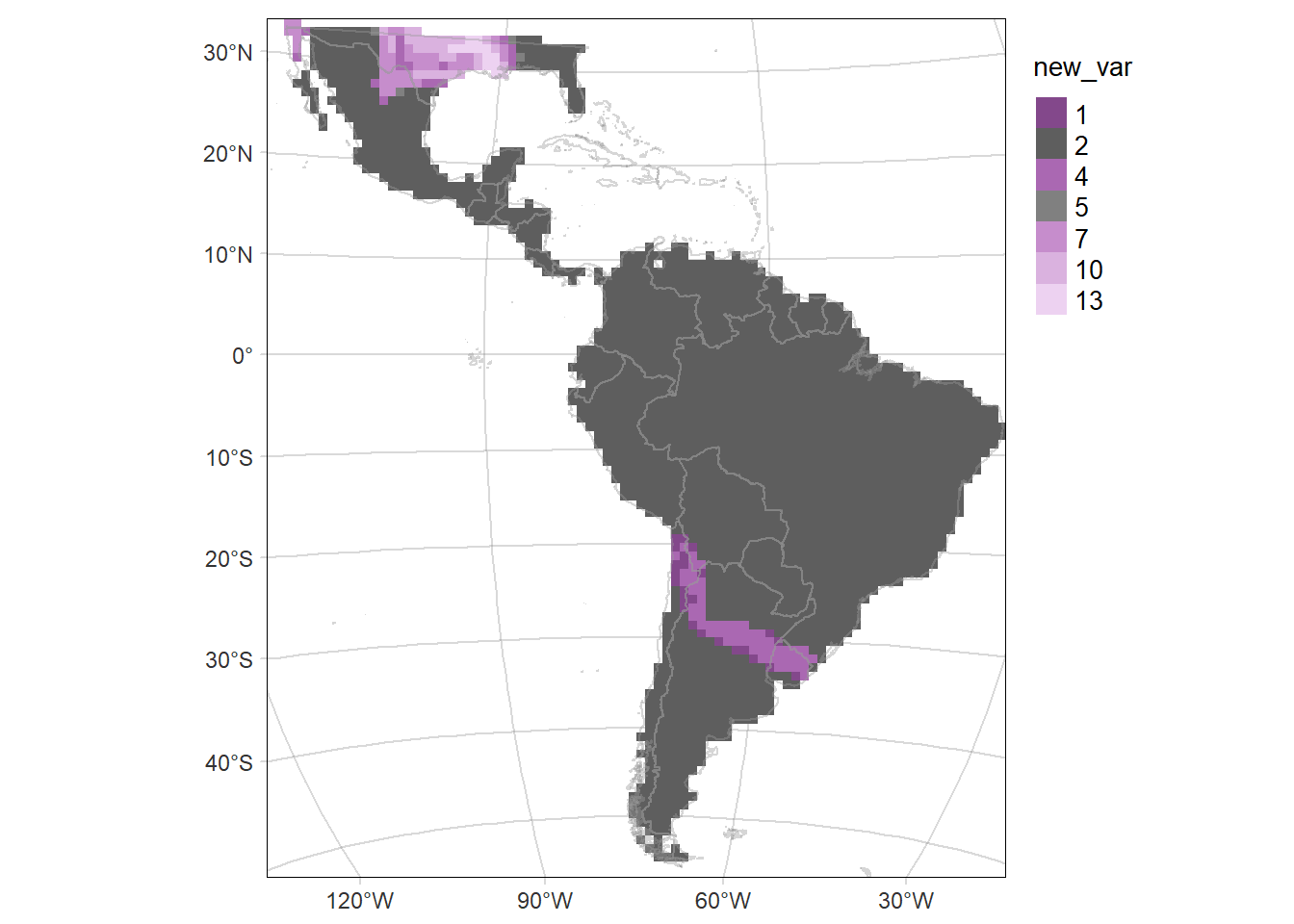
Countries thinning
Code
countryLevels <- cats(latam_countries)[[1]] #%>% mutate(value=value+1)
rasterLevels <- levels(as.factor(PO_time1_time2$country))
countries_latam <- countryLevels %>% filter(value %in% rasterLevels) %>%
  mutate(numLevel=1:length(rasterLevels)) %>% rename(country=countries)

fitted.model.ggs.alpha <- ggmcmc::ggs(fitted.model.mcmc, family="^alpha")
ci.alpha <- ci(fitted.model.ggs.alpha)

country_acce <- bind_rows(ci.alpha[length(rasterLevels)+1,],
          tibble(countries_latam, ci.alpha[1:length(rasterLevels),])) %>%
  dplyr::select(-c(value, numLevel))

#accessibility range for predictions
accessValues <- seq (0,0.5,by=0.01)

#get common steepness
commonSlope <- country_acce$median[country_acce$Parameter=="alpha1"]

#write function to get predictions for a given country
getPreds <- function(country){
  #get country intercept
  countryIntercept = country_acce$median[country_acce$country==country & !is.na(country_acce$country)]
  #return all info
  data.frame(country = country,
             access = accessValues,
             preds= countryIntercept * exp(((-1 * commonSlope)*accessValues)))
}

allPredictions <- country_acce %>%
                  filter(!is.na(country)) %>%
                  filter(country %in% countries$iso_a2) %>%
                  pull(country) %>%
                  map_dfr(getPreds)

allPredictions <- left_join(as_tibble(allPredictions),
                            countries %>% select(country=iso_a2, name_en) %>%
                              st_drop_geometry(), by='country') %>%
  filter(country!='VG' & country!= 'TT' & country!= 'FK' & country!='AW')

# just for exploration - easier to see which county is doing which
acce_country <- ggplot(allPredictions)+
    geom_line(aes(x = access, y  = preds, colour = name_en), show.legend = F) +
    viridis::scale_color_viridis(option = 'turbo', discrete=TRUE) +
    theme_bw() +
    facet_wrap(~name_en, ncol = 5) +
    ylab("Probability of retention") + xlab("Accessibility")

acce_country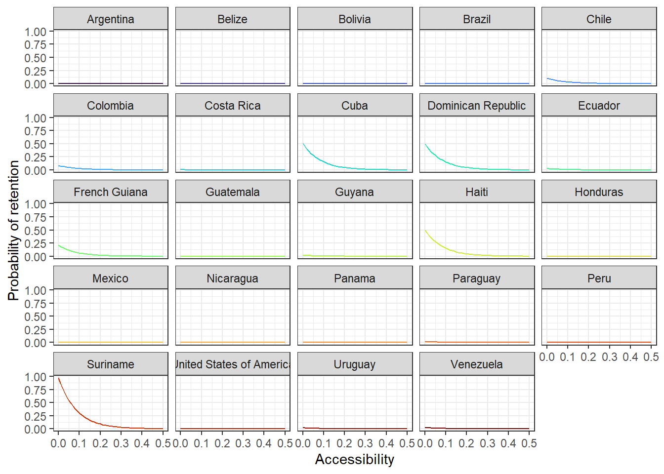
Code
# all countries
acce_allcountries <- ggplot(allPredictions) +
  geom_line(aes(x = access, y  = preds, colour = name_en), show.legend = F)+
  viridis::scale_color_viridis(option = 'turbo', discrete=TRUE) +
  theme_bw() +
  ylab("Probability of retention") + xlab("Accessibility")

acce_allcountries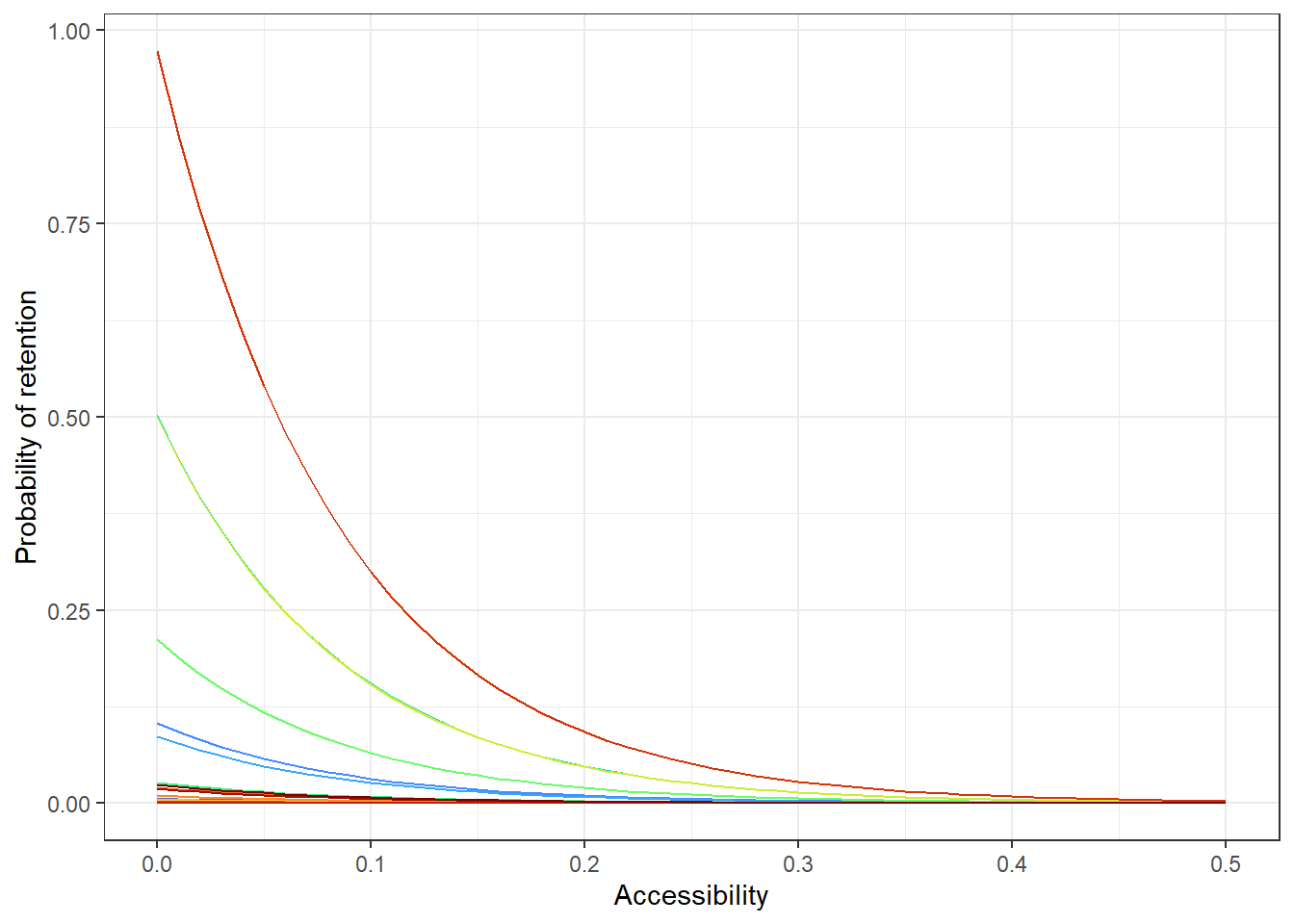
Effect of the environmental covariates on the intensity of the point process
Code
caterpiller.params <- fitted.model.ggs.b %>%
  filter(grepl('env', Parameter)) %>%
  mutate(Parameter=as.factor(ifelse(Parameter=='env.bio_10', 'mean temperature of warmest quarter',
                                    ifelse(Parameter=='env.tree', 'percentage of tree cover',
                                           ifelse(Parameter=='env.npp', 'npp',
                                                  ifelse(Parameter=='env.bio_17', 'precipitation of driest quarter', Parameter)))))) %>%
  ggs_caterpillar(line=0) +
  theme_light() +
  labs(y='', x='posterior densities')

caterpiller.params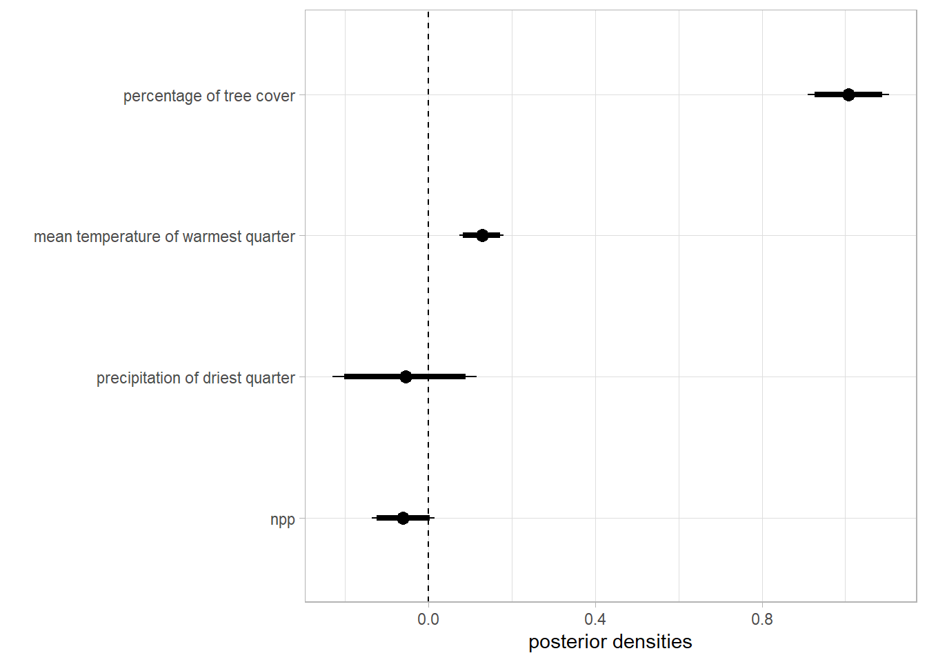
Boxplot of posterior densities of the predicted area in both time periods
Code
fitted.model.ggs.A <- ggmcmc::ggs(fitted.model.mcmc,  family="^A")

# CI
ggmcmc::ci(fitted.model.ggs.A)
# A tibble: 2 x 6
Parameter low Low median High high
<fct> <dbl> <dbl> <dbl> <dbl> <dbl>
1 A.time1 1808. 1814. 1841. 1867. 1872.
2 A.time2 1760. 1764. 1787. 1812. 1817.Code
fitted.model$BUGSoutput$summary['A.time2',] mean sd 2.5% 25% 50% 75%
1787.313361 14.545086 1760.359918 1777.205587 1786.821867 1796.824127
97.5% Rhat n.eff
1817.302039 1.001234 7600.000000 Code
# fitted.model$BUGSoutput$mean$A.time2
fitted.model$BUGSoutput$summary['A.time1',]
mean sd 2.5% 25% 50% 75%
1840.509025 16.381823 1808.470679 1829.216382 1840.575059 1851.840485
97.5% Rhat n.eff
1872.194239 1.001212 8300.000000 Code
# fitted.model$BUGSoutput$mean$A.time1

# boxplot
range.boxplot <- ggs_caterpillar(fitted.model.ggs.A, horizontal=FALSE, ) + theme_light(base_size = 14) +
    labs(y='', x='Area (number of 100x100 km grid-cells)')

range.boxplot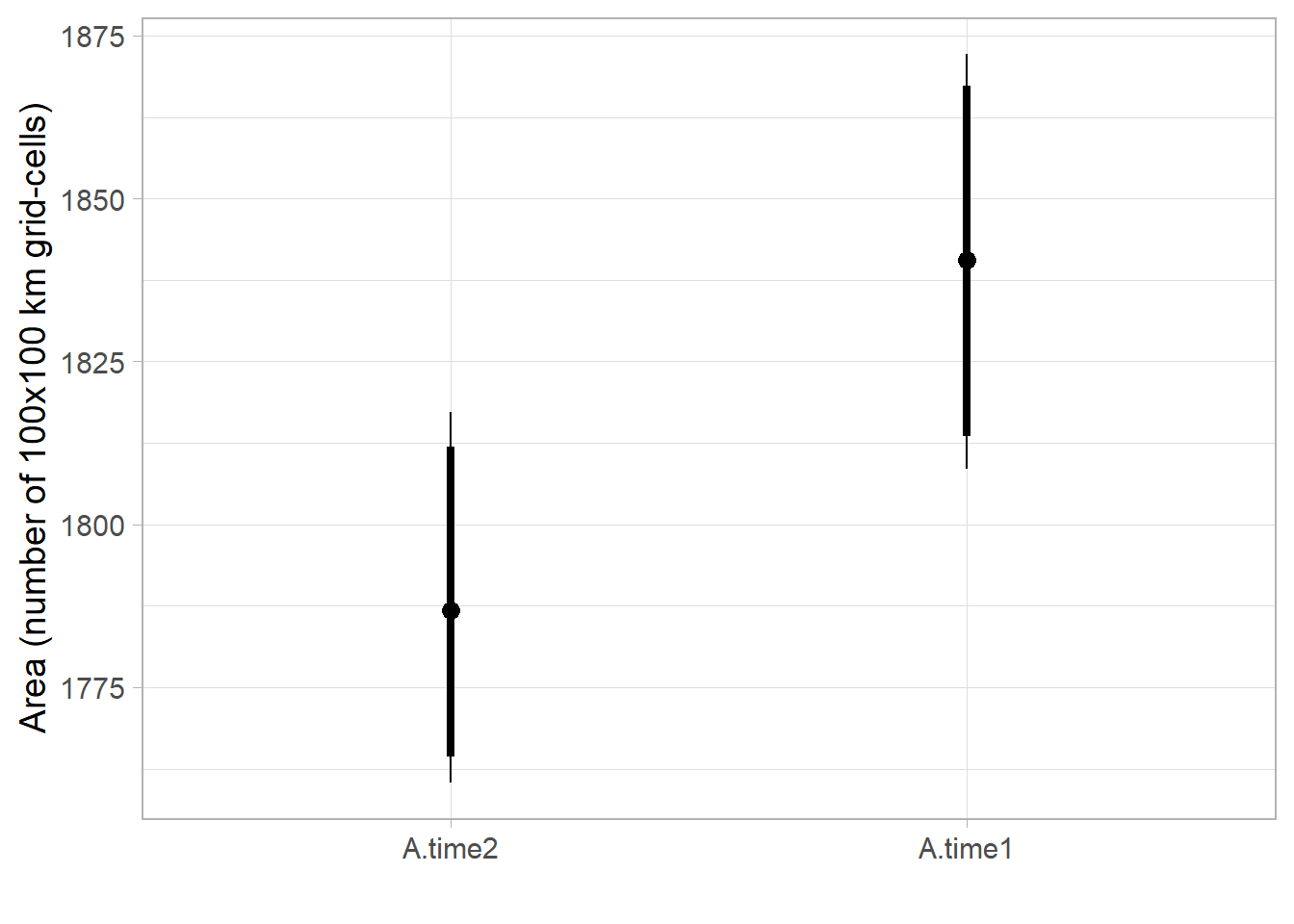
Code
# CI
range.ci <- ggmcmc::ci(fitted.model.ggs.A) %>%
    mutate(Parameter = fct_rev(Parameter)) %>%
    ggplot(aes(x = Parameter, y = median, ymin = low, ymax = high)) +
    geom_boxplot(orientation = 'y', size=1) +
    stat_summary(fun=mean, geom="point",
                 shape=19, size=4, show.legend=FALSE) +
    theme_light(base_size = 14) +
    labs(x='', y='Area (number of 100x100 km grid-cells)')

range.ci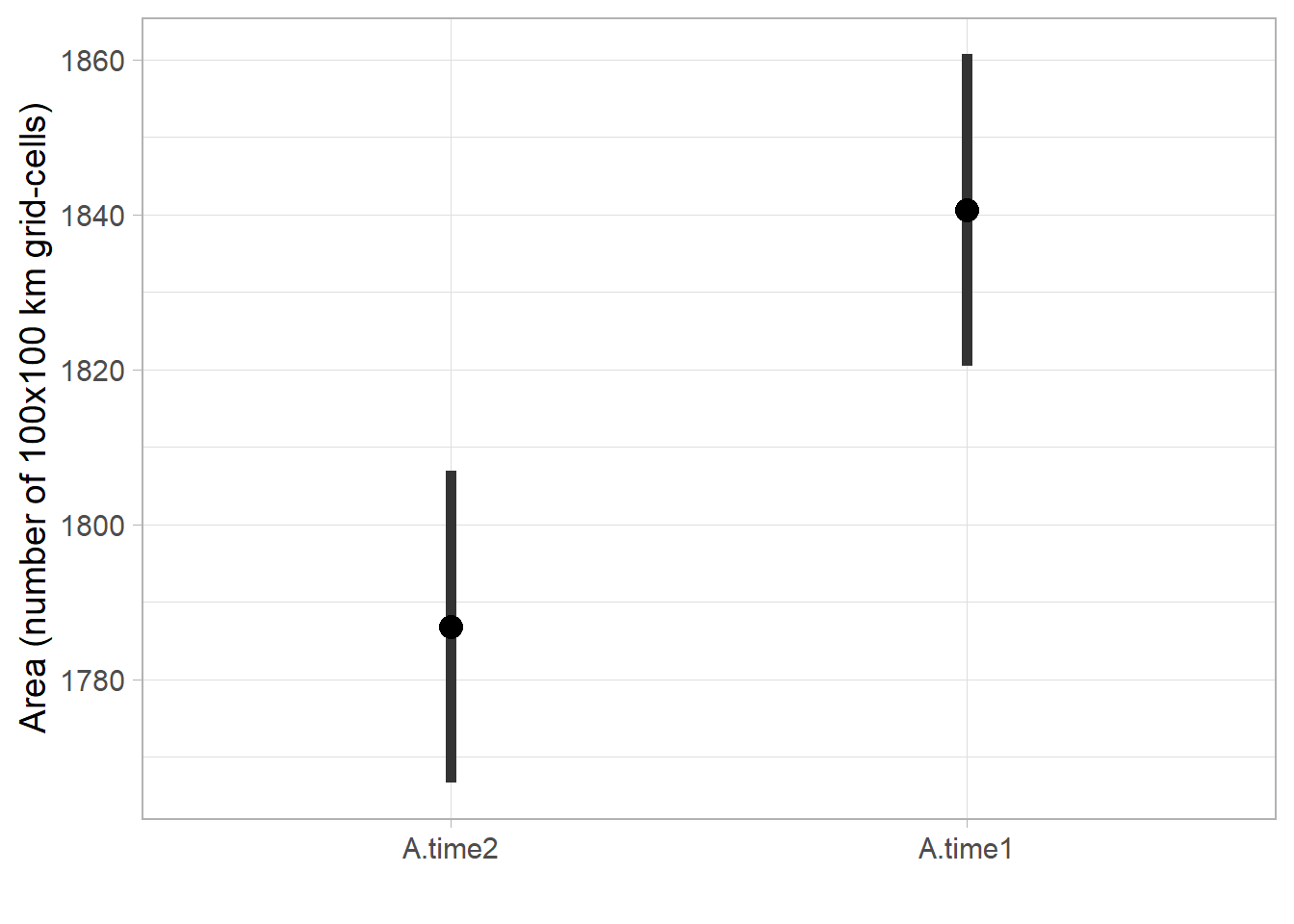
posterior distribution of range change (Area).
Code
fitted.model.ggs.delta.A <- ggmcmc::ggs(fitted.model.mcmc,  family="^delta.A")

# CI
ggmcmc::ci(fitted.model.ggs.delta.A)
# A tibble: 1 x 6
Parameter low Low median High high
<fct> <dbl> <dbl> <dbl> <dbl> <dbl>
1 delta.A -64.3 -62.5 -53.2 -43.9 -42.1Code
fitted.model$BUGSoutput$summary['delta.A',] mean sd 2.5% 25% 50% 75%
-53.195664 5.658175 -64.273671 -57.034517 -53.199618 -49.402629
97.5% Rhat n.eff
-42.131519 1.002259 1600.000000 Code
#densitiy
delta.A.plot <- fitted.model.ggs.delta.A %>% group_by(Iteration) %>%
    summarise(area=median(value)) %>%
    ggplot(aes(area)) +
    geom_density(col='grey30', fill='black', alpha = 0.3, size=1) +
    scale_y_continuous(breaks=c(0,0.0025,0.005, 0.0075, 0.01, 0.0125)) +
    geom_abline(intercept = 0, slope=1, linetype=2, size=1) +
    # vertical lines at 95% CI
    stat_boxplot(geom = "vline", aes(xintercept = ..xmax..), size=0.5, col='red') +
    stat_boxplot(geom = "vline", aes(xintercept = ..xmiddle..), size=0.5, col='red') +
    stat_boxplot(geom = "vline", aes(xintercept = ..xmin..), size=0.5, col='red') +
    theme_light(base_size = 14, base_line_size = 0.2) +
    labs(y='Probability density', x=expression(Delta*'Area'))

delta.A.plot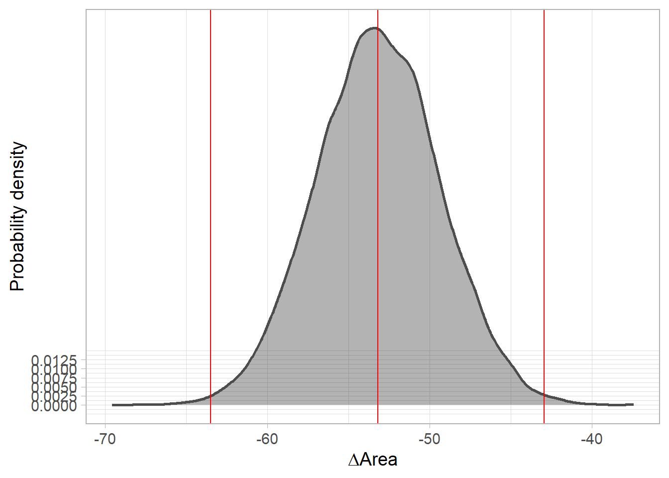
posterior predictive checks
PO
Expected vs observed
Code
counts <- PO_time1_time2$count
counts.new <- fitted.model$BUGSoutput$mean$y.PO.new
lambda <- fitted.model$BUGSoutput$mean$lambda
pred.PO <- data.frame(counts, counts.new, lambda)

# fitted.model$BUGSoutput$summary['fit.PO',]
# fitted.model$BUGSoutput$summary['fit.PO.new',]

pp.PO <- ggplot(pred.PO, aes(x=counts, y=lambda), fill=NA) +
    geom_point(size=3, shape=21)  +
    xlim(c(0, 100)) +
    ylim(c(0, 50)) +
    labs(x='observed', y=expression(lambda), title='Presence-only') +
    geom_abline(col='red') +
    theme_bw()

pp.PO.log10 <- ggplot(pred.PO, aes(x=counts, y=lambda), fill=NA) +
    geom_point(size=3, shape=21)  +
    scale_x_log10(limits=c(0.01, 100)) +
    scale_y_log10(limits=c(0.01, 100)) +
    coord_fixed(ratio=1) +
    labs(x='observed (log scale)', y=expression(lambda*'(log scale)'), title='log10 scale') +
    geom_abline(col='red') +
    theme_bw()

pp.PO | pp.PO.log10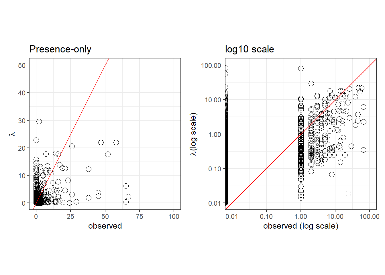
Residual Diagnostics
Code
library(DHARMa)

simulations <- fitted.model$BUGSoutput$sims.list$y.PO.new
pred <- apply(fitted.model$BUGSoutput$sims.list$lambda, 2, median)
#dim(simulations)

sim <- createDHARMa(simulatedResponse = t(simulations),
                    observedResponse = PO_time1_time2$count,
                    fittedPredictedResponse = pred,
                    integerResponse = T)

plotSimulatedResiduals(sim)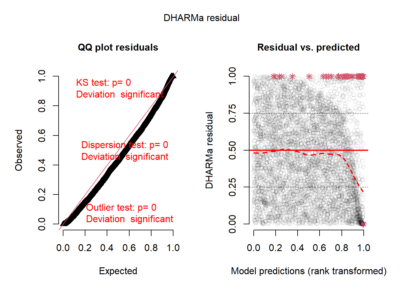
Grid-level change
Code
range_change <- as_tibble(rast2[PO_time2$pixel] - rast1[PO_time2$pixel]) %>% rename(range=time2)
numRecord_change <- as_tibble(PO_time2$count - PO_time1$count) %>% rename(numRecord=value)

grid.level.change <- bind_cols(range_change, numRecord_change) %>%
    mutate(nonzero=ifelse(numRecord==0, '0', '>=1')) %>%
    ggplot() +
    geom_point(aes(y=range, x=numRecord, col=nonzero), size=1) +
    geom_vline(xintercept=0, linetype=2, size=0.5) +
    geom_hline(yintercept=0, linetype=2, size=0.5) +
    labs(y = expression('Predicted grid-level range change (Ppred'['time2']*'-Ppred'['time1']*')'),
         x= expression('Grid-level range change in number of records (Nrecords'['time2']*'-Nrecords'['time1']*')'),
         col = 'Number of records\nper grid cell') +
    theme_bw(base_size = 14)

grid.level.change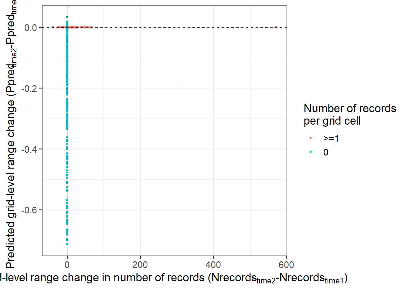
PA
Tjur R2
Code
presabs <- PA_time1_time2$presabs
psi <- fitted.model$BUGSoutput$mean$psi
pred.PA <- data.frame(presabs, psi)

r2_tjur <- round(fitted.model$BUGSoutput$mean$r2_tjur, 3)
fitted.model$BUGSoutput$summary['r2_tjur',]
mean sd 2.5% 25% 50%
0.271592716 0.002618364 0.266388400 0.269821764 0.271624340
75% 97.5% Rhat n.eff
0.273384699 0.276629291 1.001746003 2600.000000000 Code
pp.PA <- ggplot(pred.PA, aes(x=presabs, y=psi, col=presabs)) +
    geom_jitter(height = 0, width = .05, size=1)  +
    scale_x_continuous(breaks=seq(0,1,0.25)) + scale_colour_binned() +
    labs(x='observed', y=expression(psi), title='Presence-absence') +
    stat_summary(
        fun = mean,
        geom = "errorbar",
        aes(ymax = ..y.., ymin = ..y..),
        width = 0.2, size=2) +
    theme_bw() + theme(legend.position = 'none')+
    annotate(geom="text", x=0.5, y=0.5,
             label=paste('Tjur R-squared = ', r2_tjur))

pp.PA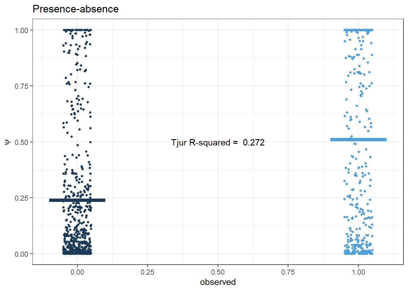
AUC
Code
auc.sens.fpr <- bind_cols(sens=fitted.model$BUGSoutput$mean$sens,
                          fpr=fitted.model$BUGSoutput$mean$fpr)

auc.value <- round(fitted.model$BUGSoutput$mean$auc, 3)

ggplot(auc.sens.fpr, aes(fpr, sens)) +
  geom_line() + geom_point() +
  labs(x='1 - Specificity', y='Sensitivity') +
  annotate(geom="text", x=0.5, y=0.5,
           label=paste('AUC = ', auc.value)) +
  theme_bw()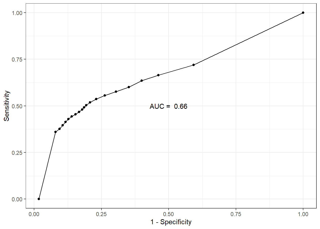
Code
fitted.model$BUGSoutput$summary['auc',] mean sd 2.5% 25% 50%
0.659947167 0.002314093 0.655368690 0.658375153 0.659975451
75% 97.5% Rhat n.eff
0.661541599 0.664355802 1.001477651 4000.000000000