Cerdocyon thous Model Outputs

Author

Florencia Grattarola

Published

September 23, 2024

Model outputs for Cerdocyon thous.

R Libraries

library(patchwork)
library(mcmcplots)
library(ggmcmc)
library(tidybayes)
library(tmap)
tmap_mode("plot")
library(terra)
library(sf)
sf::sf_use_s2(FALSE)
library(tidyverse)
# options
options(scipen = 999)

Basemaps

equalareaCRS <-  '+proj=laea +lon_0=-73.125 +lat_0=0 +datum=WGS84 +units=m +no_defs'
latam <- st_read('data/latam.gpkg', layer = 'latam', quiet = T)
countries <- st_read('data/latam.gpkg', layer = 'countries', quiet = T)
latam_land <- st_read('data/latam.gpkg', layer = 'latam_land', quiet = T)
latam_raster <- rast('data/latam_raster.tif', lyrs='latam')
latam_countries <- rast('data/latam_raster.tif', lyrs='countries')

cthous_IUCN <- sf::st_read('big_data/cthous_IUCN.shp', quiet = T) %>% sf::st_transform(crs=equalareaCRS)

Species data and covariates

# Presence-absence data
cthous_expert_blob_time1 <- readRDS('data/species_POPA_data/cthous_expert_blob_time1.rds')
cthous_expert_blob_time2 <- readRDS('data/species_POPA_data/cthous_expert_blob_time2.rds')

PA_time1 <- readRDS('data/species_POPA_data/data_cthous_PA_time1.rds') %>%
  cbind(expert=cthous_expert_blob_time1) %>%
  filter(!is.na(env.bio_16) &!is.na(env.bio_19) & !is.na(env.npp) & !is.na(env.tree) & !is.na(expert)) # remove NA's
PA_time2 <- readRDS('data/species_POPA_data/data_cthous_PA_time2.rds') %>%
  cbind(expert=cthous_expert_blob_time2) %>% 
  filter(!is.na(env.bio_16) &!is.na(env.bio_19) & !is.na(env.npp) & !is.na(env.tree) & !is.na(expert)) # remove NA's

# Presence-only data
cthous_expert_gridcell <- readRDS('data/species_POPA_data/cthous_expert_gridcell.rds')

PO_time1 <- readRDS('data/species_POPA_data/data_cthous_PO_time1.rds') %>%
  cbind(expert=cthous_expert_gridcell$dist_exprt) %>% 
  filter(!is.na(env.bio_16) &!is.na(env.bio_19) & !is.na(env.npp) & !is.na(env.tree) & !is.na(acce) & !is.na(count) & !is.na(expert)) # remove NA's
PO_time2  <- readRDS('data/species_POPA_data/data_cthous_PO_time2.rds')  %>%
  cbind(expert=cthous_expert_gridcell$dist_exprt) %>% 
  filter(!is.na(env.bio_16) &!is.na(env.bio_19) & !is.na(env.npp) & !is.na(env.tree) & !is.na(acce) & !is.na(count) & !is.na(expert)) # remove NA's

PA_time1_time2 <- rbind(PA_time1 %>% mutate(time=1), PA_time2 %>% mutate(time=2)) 
PO_time1_time2 <- rbind(PO_time1 %>% mutate(time=1), PO_time2 %>% mutate(time=2))

Read model

fitted.model <- readRDS('D:/Flo/JAGS_models/cthous_model.rds') # deleted after model output
# fitted.model <- readRDS('big_data/cthous_model.rds') # deleted after model output

# as.mcmc.rjags converts an rjags Object to an mcmc or mcmc.list Object.
fitted.model.mcmc <- mcmcplots::as.mcmc.rjags(fitted.model)

Model diagnostics

The fitted.model is an object of class rjags.

Code

# labels for the linear predictor `b`
L.fitted.model.b <- plab("b", 
                         list(Covariate = c('Intercept', 
                                            'env.bio_16',
                                            'env.bio_19',
                                            'env.npp', 
                                            'env.tree', 
                                            'expert',
                                            sprintf('spline%i', 1:16)))) # changes with n.spl

# tibble object for the linear predictor `b` extracted from the rjags fitted model
fitted.model.ggs.b <- ggmcmc::ggs(fitted.model.mcmc, 
                                  par_labels = L.fitted.model.b,
                                  family="^b\\[")

# diagnostics
ggmcmc::ggmcmc(fitted.model.ggs.b, file="docs/cthous_model_diagnostics.pdf", param_page=3)

Plotting histograms

Plotting density plots

Plotting traceplots

Plotting running means

Plotting comparison of partial and full chain

Plotting autocorrelation plots

Plotting crosscorrelation plot

Plotting Potential Scale Reduction Factors

Plotting shrinkage of Potential Scale Reduction Factors

Plotting Number of effective independent draws

Plotting Geweke Diagnostic

Plotting caterpillar plot

Time taken to generate the report: 32 seconds.

Traceplot

Code

ggs_traceplot(fitted.model.ggs.b)

Rhat

Code

ggs_Rhat(fitted.model.ggs.b)

Probability of occurrence of Cerdocyon thous

For each period: time1 and time2, and their difference (time2-time1)

Code

P.pred <- fitted.model$BUGSoutput$mean$P.pred
preds <- data.frame(PO_time1_time2, P.pred)
preds1 <- preds[preds$time == 1,]
preds2 <- preds[preds$time == 2,]

rast <- latam_raster
rast[] <- NA
rast1 <- rast2 <- terra::rast(rast)

rast1[preds1$pixel] <- preds1$P.pred
rast2[preds2$pixel] <- preds2$P.pred

rast1 <- rast1 %>% terra::mask(., vect(latam_land))
rast2 <- rast2 %>% terra::mask(., vect(latam_land))
names(rast1) <- 'time1'
names(rast2) <- 'time2'

# Map of the of the probability of occurrence in the first period (time1: 2000-2013)
time1MAP <- tm_graticules(alpha = 0.3) +  
    tm_shape(rast1) +
    tm_raster(palette = 'Oranges', midpoint = NA, style= "cont")  + 
    tm_shape(countries) +
    tm_borders(col='grey60', alpha = 0.4) + 
    tm_layout(legend.outside = T, frame.lwd = 0.3, scale=1.2, legend.outside.size = 0.1)

# Map of the of the probability of occurrence in the second period (time2: 2014-2021)
time2MAP <- tm_graticules(alpha = 0.3) +  
    tm_shape(rast2) +
    tm_raster(palette = 'Purples', midpoint = NA, style= "cont")  + 
    tm_shape(countries) +
    tm_borders(col='grey60', alpha = 0.4) + 
    tm_layout(legend.outside = T, frame.lwd = 0.3, scale=1.2, legend.outside.size = 0.1)

# Map of the of the change in the probability of occurrence (time2 - time1)
diffMAP <- tm_graticules(alpha = 0.3) + 
    tm_shape(rast2 - rast1) +
    tm_raster(palette = 'PiYG', midpoint = 0, style= "cont", ) +
    tm_shape(countries) +
    tm_borders(col='grey60', alpha = 0.4) + 
    tm_layout(legend.outside = T, frame.lwd = 0.3, scale=1.2, legend.outside.size = 0.1)

time1MAP

Code

time2MAP

Code

diffMAP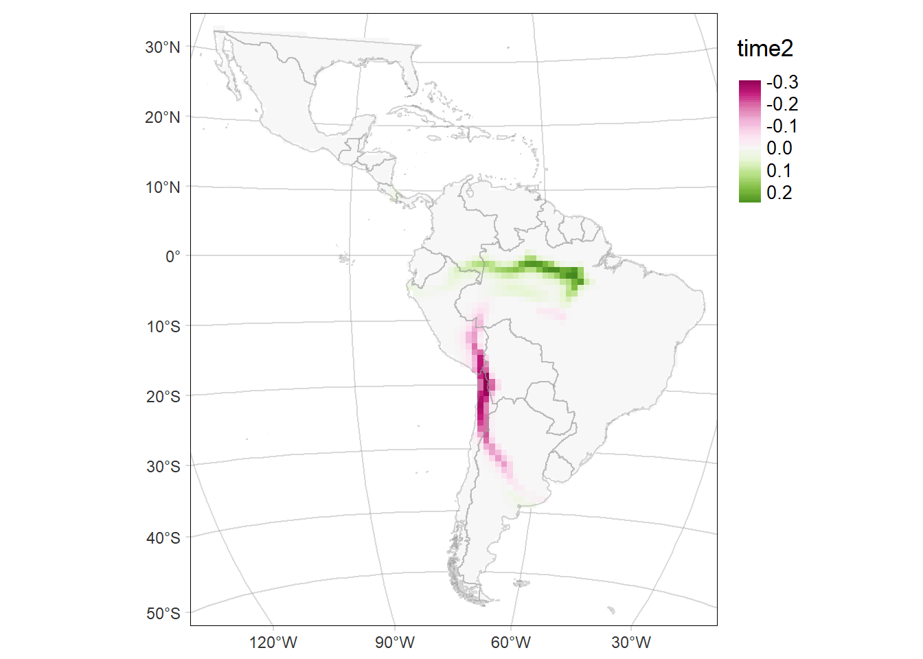

Code

tmap::tmap_save(tm = time1MAP, filename = 'docs/figs/time1MAP_SR_cthous.svg', device = svglite::svglite)
tmap::tmap_save(tm = time2MAP, filename = 'docs/figs/time2MAP_SR_cthous.svg', device = svglite::svglite)

Standard deviation (SD) of the probability of occurrence of Cerdocyon thous

Code

P.pred.sd <- fitted.model$BUGSoutput$sd$P.pred
preds.sd <- data.frame(PO_time1_time2, P.pred.sd)

preds1.sd <- preds.sd[preds.sd$time == 1,]
preds2.sd <- preds.sd[preds.sd$time == 2,]

rast.sd <- terra::rast(latam_raster)
rast.sd[] <- NA
rast1.sd <- rast2.sd <- terra::rast(rast.sd)

rast1.sd[preds1.sd$pixel] <- preds1.sd$P.pred.sd
rast2.sd[preds2.sd$pixel] <- preds2.sd$P.pred.sd

rast1.sd <- rast1.sd %>% terra::mask(., vect(latam_land))
rast2.sd <- rast2.sd %>% terra::mask(., vect(latam_land))
names(rast1.sd) <- 'time1.sd'
names(rast2.sd) <- 'time2.sd'

# Map of the SD of the probability of occurrence of the area time1 
time1MAP.sd <- tm_graticules(alpha = 0.3) +  
    tm_shape(rast1.sd) +
    tm_raster(palette = 'Oranges', midpoint = NA, style= "cont")  + 
    tm_shape(countries) +
    tm_borders(alpha = 0.3) + 
    tm_layout(legend.outside = T, frame.lwd = 0.3, scale=1.2, legend.outside.size = 0.1)

# Map of the SD of the probability of occurrence of the area time2
time2MAP.sd <-  tm_graticules(alpha = 0.3) +  
    tm_shape(rast2.sd) +
    tm_raster(palette = 'Purples', midpoint = NA, style= "cont")  + 
    tm_shape(countries) +
    tm_borders(alpha = 0.3) + 
    tm_layout(legend.outside = T, frame.lwd = 0.3, scale=1.2, legend.outside.size = 0.1)

time1MAP.sd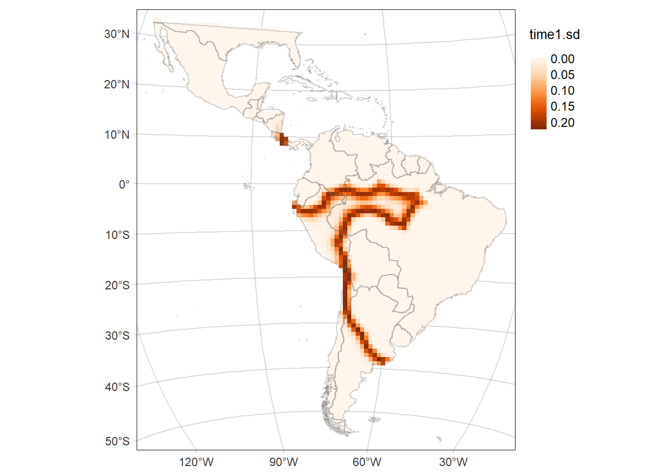

Code

time2MAP.sd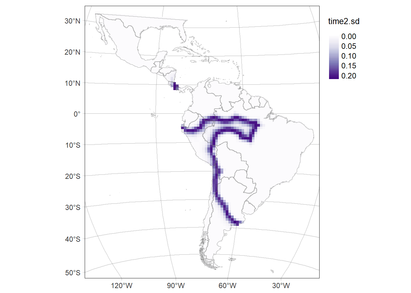

Bivariate map

Map of the difference including the Standard deviation (SD) of the probability of occurrence as the transparency of the layer.

Code

library(cols4all)
library(pals)
library(classInt)
library(stars)

bivcol = function(pal, nx = 3, ny = 3){
  tit = substitute(pal)
  if (is.function(pal))
    pal = pal()
  ncol = length(pal)
  if (missing(nx))
    nx = sqrt(ncol)
  if (missing(ny))
    ny = nx
  image(matrix(1:ncol, nrow = ny), axes = FALSE, col = pal, asp = 1)
  mtext(tit)
}

cthous.pal.pu_gn_bivd <- c4a("pu_gn_bivd", n=3, m=5)
cthous.pal <- c(t(apply(cthous.pal.pu_gn_bivd, 2, rev)))

###

pred.P.sd <- fitted.model$BUGSoutput$sd$delta.Grid
preds.sd <- data.frame(PO_time1_time2, pred.P.sd=rep(pred.P.sd, 2))

rast.sd <- terra::rast(latam_raster)
rast.sd[] <- NA
rast.sd <- terra::rast(rast.sd)

rast.sd[preds.sd$pixel] <- preds.sd$pred.P.sd
rast.sd <- rast.sd %>% terra::mask(., vect(latam_land))
names(rast.sd) <- c('diff')

# Map of the SD of the probability of occurrence of the area time2
delta.GridMAP.sd <-  tm_graticules(alpha = 0.3) +  
    tm_shape(rast.sd) +
    tm_raster(palette = 'Greys', midpoint = NA, style= "cont")  + 
    tm_shape(countries) +
    tm_borders(alpha = 0.3) + 
    tm_layout(legend.outside = T, frame.lwd = 0.3, scale=1.2, legend.outside.size = 0.1)

delta.GridMAP.sd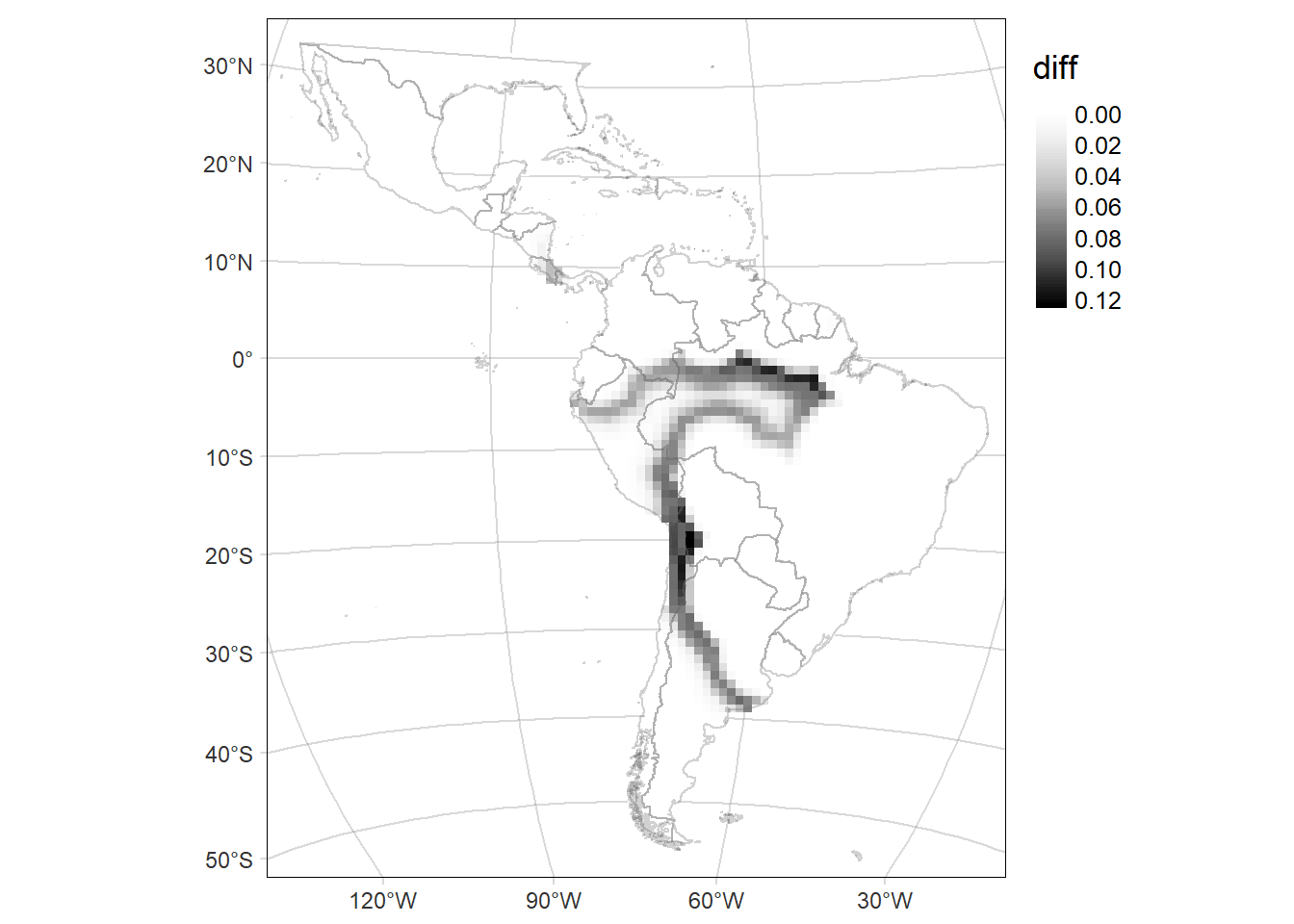

Code

rast.stars <- c(stars::st_as_stars(rast2-rast1), stars::st_as_stars(rast.sd))
names(rast.stars) <- c('diff', 'sd')

par(mfrow=c(2,2))
hist(rast1)
hist(rast2)
hist(rast.stars['diff'])
hist(rast.stars['sd'])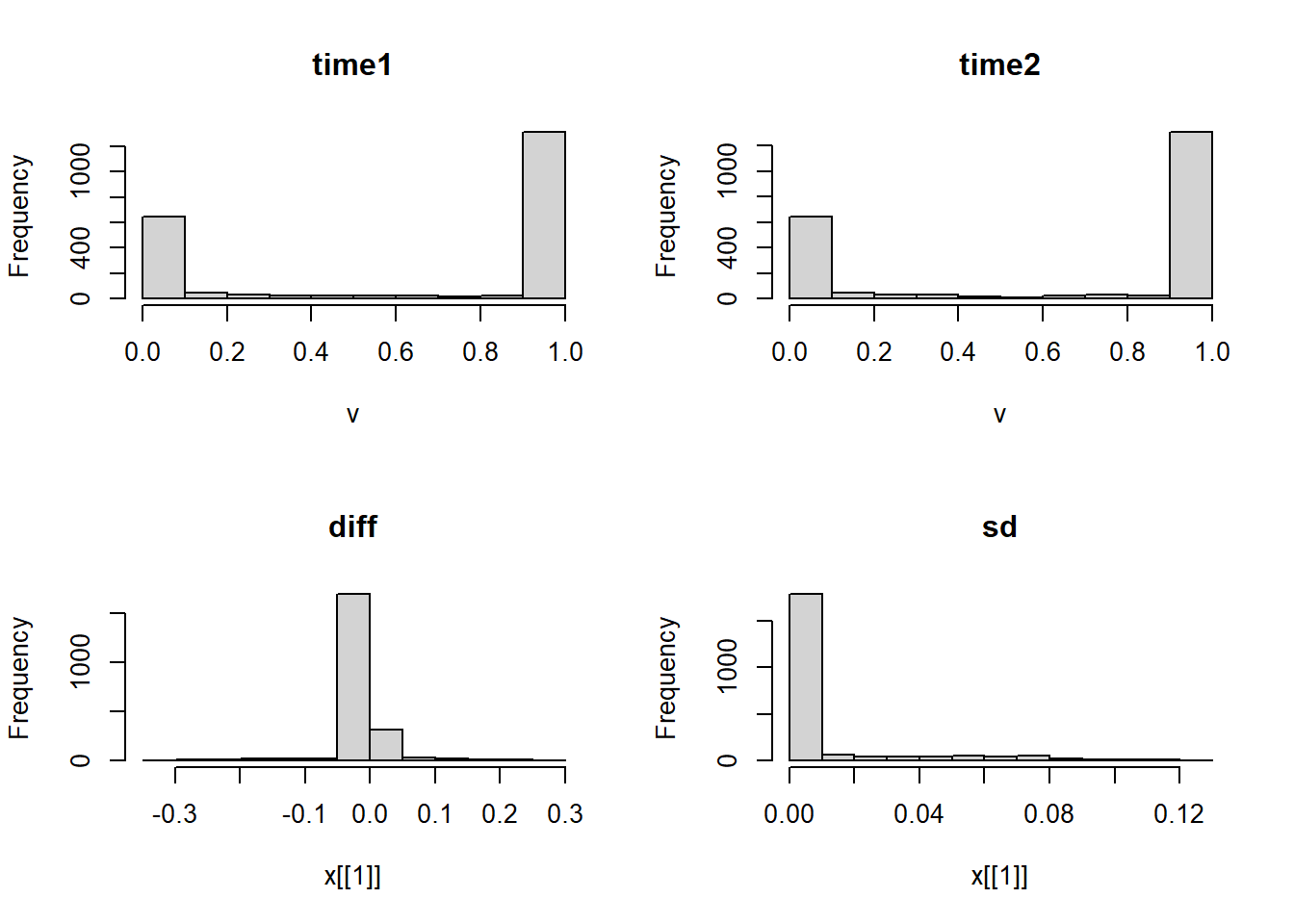

Code

par(mfrow=c(1,1))

add_new_var = function(x, var1, var2, nbins1, nbins2, style1, style2,fixedBreaks1, fixedBreaks2){
  class1 = suppressWarnings(findCols(classIntervals(c(x[[var1]]), 
                                                    n = nbins1, 
                                                    style = style1,
                                                    fixedBreaks1=fixedBreaks1)))
  
  class2 = suppressWarnings(findCols(classIntervals(c(x[[var2]]), 
                                                    n = nbins2, 
                                                    style = style2,
                                                    fixedBreaks=fixedBreaks2)))
  
  x$new_var = class1 + nbins1 * (class2 - 1)
  return(x)
}

rast.bivariate = add_new_var(rast.stars,
                             var1 = "diff", 
                             var2 = "sd",
                             nbins1 = 3, 
                             nbins2 = 5, 
                             style1 = "fixed",
                             fixedBreaks1=c(-1,-0.05, 0.05, 1),
                             style2 = "fixed",
                             fixedBreaks2=c(0, 0.05, 0.1, 0.15, 0.2, 0.3))


# See missing classes and update palette
all_classes <- seq(1,15,1)
rast_classes <- as_tibble(rast.bivariate['new_var']) %>% 
    distinct(new_var) %>% filter(!is.na(new_var)) %>% pull()
absent_classes <- all_classes[!(all_classes %in% rast_classes)]

if (length(absent_classes)==0){
  cthous.new.pal <- cthous.pal
} else cthous.new.pal <- cthous.pal[-c(absent_classes)]

# Map of the of the change in the probability of occurrence (time2 - time1)
# according to the mean SD of the probability of occurrence  (mean(time2.sd, time1.sd))

diffMAP.SD <- tm_graticules(alpha = 0.3) + 
  tm_shape(rast.bivariate) +
  tm_raster("new_var", style= "cat", palette = cthous.new.pal) +
  tm_shape(countries) +
  tm_borders(col='grey60', alpha = 0.4) + 
  tm_layout(legend.outside = T, frame.lwd = 0.3, scale=1.2, legend.outside.size = 0.1)

diffMAP.SD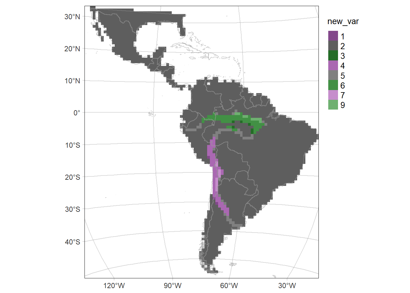

Code

tmap::tmap_save(tm = diffMAP.SD, filename = 'docs/figs/diffMAP_SD_cthous.svg', device = svglite::svglite)

Countries thinning

Code

countryLevels <- cats(latam_countries)[[1]] #%>% mutate(value=value+1)
rasterLevels <- levels(as.factor(PO_time1_time2$country))
countries_latam <- countryLevels %>% filter(value %in% rasterLevels) %>% 
  mutate(numLevel=1:length(rasterLevels)) %>% rename(country=countries)

fitted.model.ggs.alpha <- ggmcmc::ggs(fitted.model.mcmc, family="^alpha")
ci.alpha <- ci(fitted.model.ggs.alpha)

country_acce <- bind_rows(ci.alpha[length(rasterLevels)+1,], 
          tibble(countries_latam, ci.alpha[1:length(rasterLevels),])) %>% 
  dplyr::select(-c(value, numLevel))

#accessibility range for predictions
accessValues <- seq (0,0.5,by=0.01)

#get common steepness
commonSlope <- country_acce$median[country_acce$Parameter=="alpha1"]

#write function to get predictions for a given country
getPreds <- function(country){
  #get country intercept
  countryIntercept = country_acce$median[country_acce$country==country & !is.na(country_acce$country)]
  #return all info
  data.frame(country = country,
             access = accessValues,
             preds= countryIntercept * exp(((-1 * commonSlope)*accessValues)))
}

allPredictions <- country_acce %>%
                  filter(!is.na(country)) %>%
                  filter(country %in% countries$iso_a2) %>% 
                  pull(country) %>%
                  map_dfr(getPreds)

allPredictions <- left_join(as_tibble(allPredictions), 
                            countries %>% select(country=iso_a2, name_en) %>% 
                              st_drop_geometry(), by='country') %>% 
  filter(country!='VG' & country!= 'TT' & country!= 'FK' & country!='AW')

# just for exploration - easier to see which county is doing which
acce_country <- ggplot(allPredictions)+
    geom_line(aes(x = access, y  = preds, colour = name_en), show.legend = F) + 
    viridis::scale_color_viridis(option = 'turbo', discrete=TRUE) +
    theme_bw() + 
    facet_wrap(~name_en, ncol = 5) + 
    ylab("Probability of retention") + xlab("Accessibility")

acce_country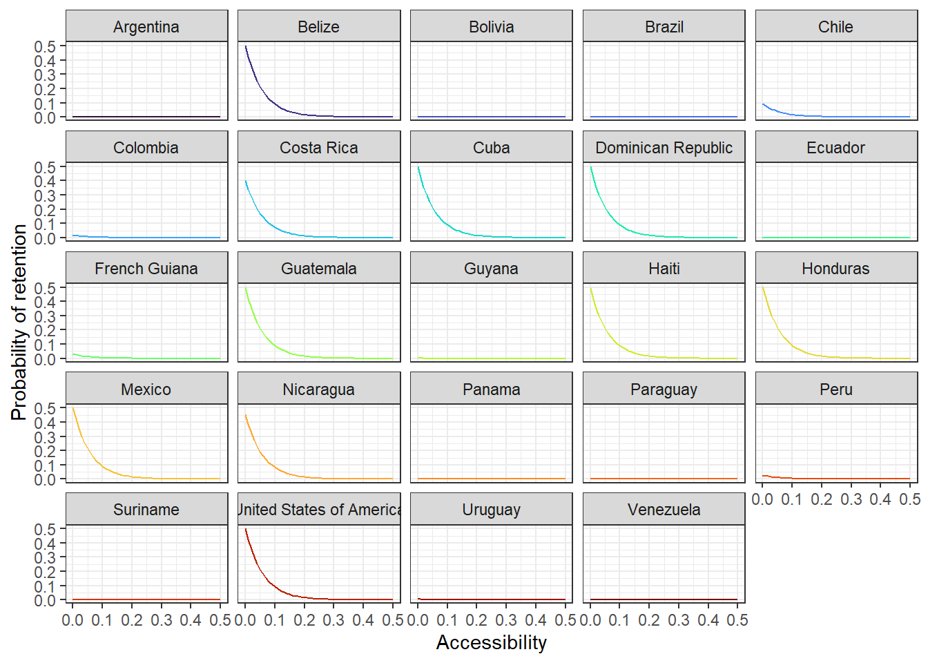

Code

# all countries
acce_allcountries <- ggplot(allPredictions) +
  geom_line(aes(x = access, y  = preds, colour = name_en), show.legend = F)+
  viridis::scale_color_viridis(option = 'turbo', discrete=TRUE) +
  theme_bw() + 
  ylab("Probability of retention") + xlab("Accessibility")

acce_allcountries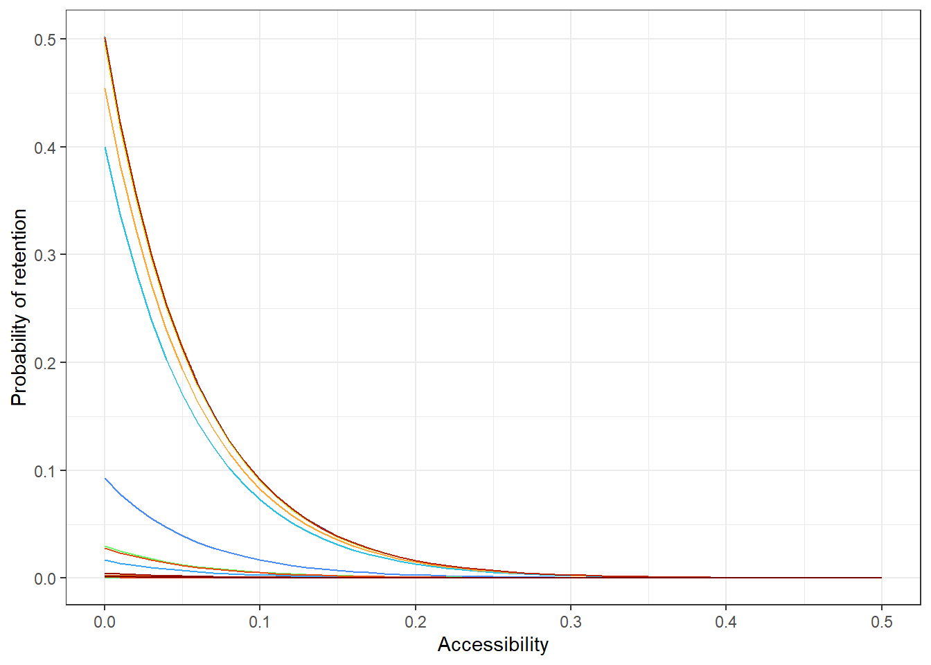

Effect of the environmental covariates on the intensity of the point process

Code

caterpiller.params <- fitted.model.ggs.b %>%
  filter(grepl('env', Parameter)) %>% 
  mutate(Parameter=as.factor(ifelse(Parameter=='env.bio_16', 'precipitation of wettest quarter',
                                    ifelse(Parameter=='env.tree', 'percentage of tree cover',
                                           ifelse(Parameter=='env.npp', 'npp',
                                                  ifelse(Parameter=='env.bio_19', 'precipitation of coldest quarter', Parameter)))))) %>% 
  ggs_caterpillar(line=0) + 
  theme_light() + 
  labs(y='', x='posterior densities')

caterpiller.params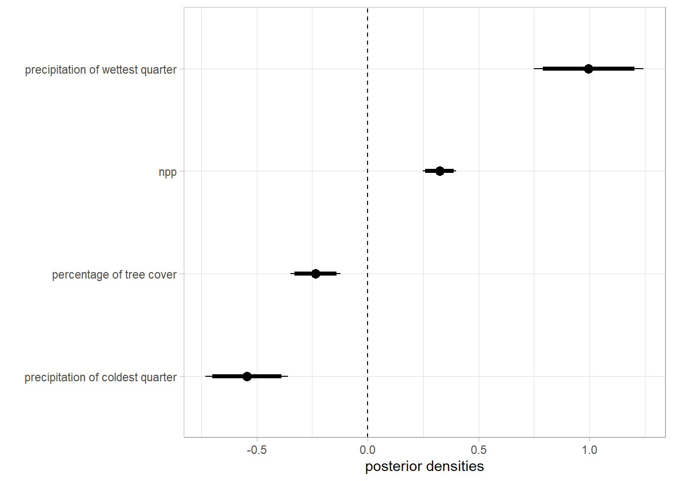

Boxplot of posterior densities of the predicted area in both time periods

Code

fitted.model.ggs.A <- ggmcmc::ggs(fitted.model.mcmc,  family="^A")

# CI
ggmcmc::ci(fitted.model.ggs.A)

# A tibble: 2 x 6
  Parameter   low   Low median  High  high
  <fct>     <dbl> <dbl>  <dbl> <dbl> <dbl>
1 A.time1   1325. 1338.  1408. 1469. 1480.
2 A.time2   1324. 1337.  1408. 1468. 1480.

Code

fitted.model$BUGSoutput$summary['A.time2',]

       mean          sd        2.5%         25%         50%         75% 
1405.796629   39.603611 1323.528844 1379.885276 1407.606718 1433.031393 
      97.5%        Rhat       n.eff 
1479.815177    1.003298  860.000000

Code

# fitted.model$BUGSoutput$mean$A.time2
fitted.model$BUGSoutput$summary['A.time1',]

       mean          sd        2.5%         25%         50%         75% 
1406.448696   39.671789 1324.706958 1380.090703 1408.422242 1434.034566 
      97.5%        Rhat       n.eff 
1479.593790    1.002962 1000.000000

Code

# fitted.model$BUGSoutput$mean$A.time1

# boxplot
range.boxplot <- ggs_caterpillar(fitted.model.ggs.A, horizontal=FALSE, ) + theme_light(base_size = 14) +
    labs(y='', x='Area (number of 100x100 km grid-cells)')

range.boxplot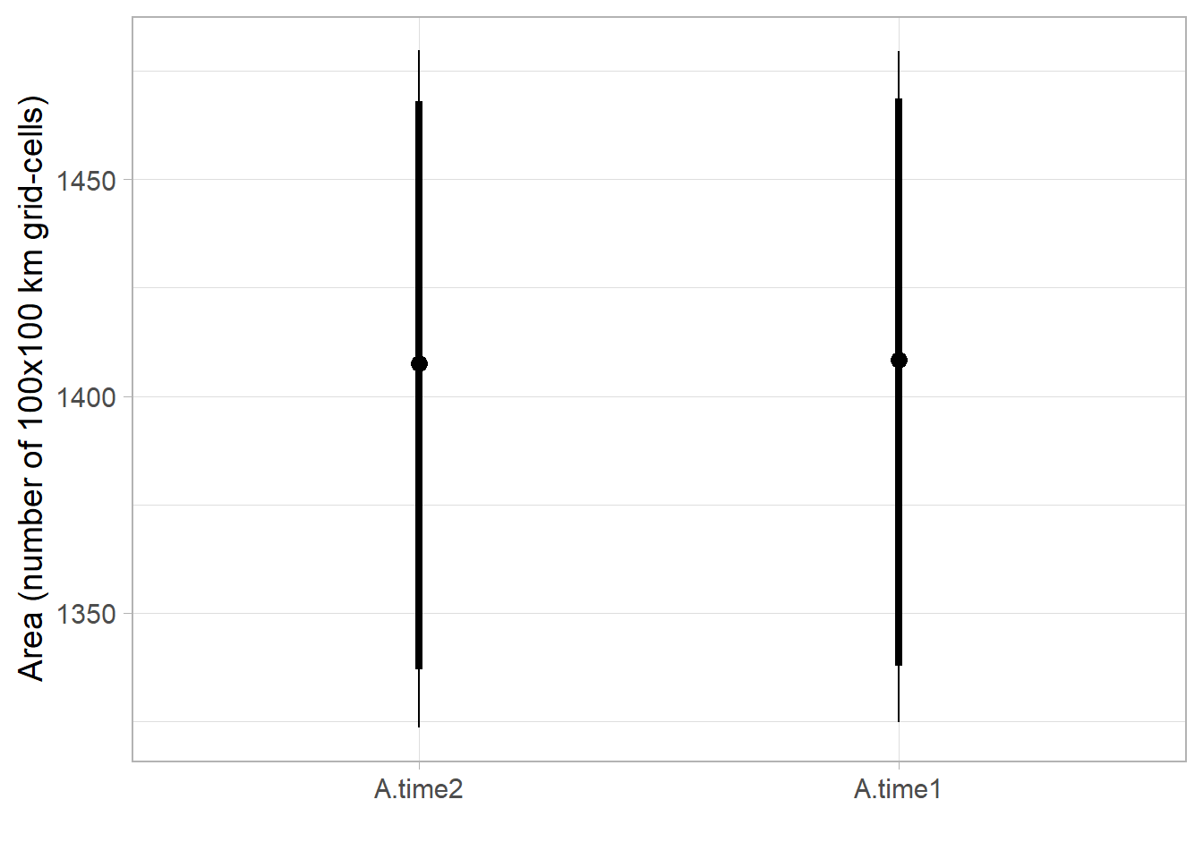

Code

# CI 
range.ci <- ggmcmc::ci(fitted.model.ggs.A) %>% 
    mutate(Parameter = fct_rev(Parameter)) %>% 
    ggplot(aes(x = Parameter, y = median, ymin = low, ymax = high)) + 
    geom_boxplot(orientation = 'y', size=1) + 
    stat_summary(fun=mean, geom="point", 
                 shape=19, size=4, show.legend=FALSE) + 
    theme_light(base_size = 14) +
    labs(x='', y='Area (number of 100x100 km grid-cells)')

range.ci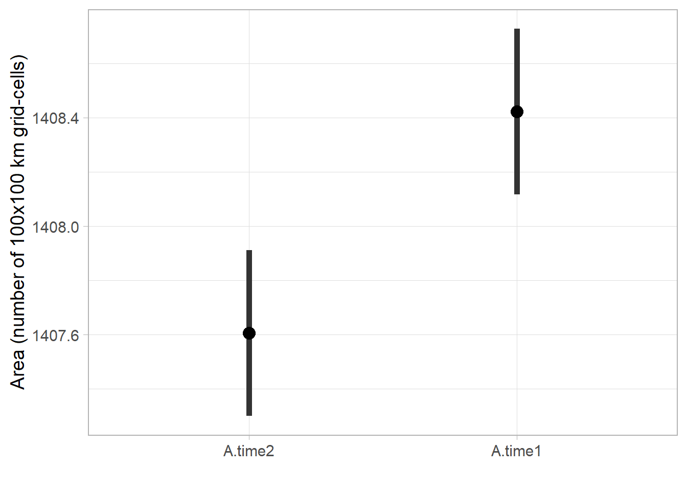

posterior distribution of range change (Area).

Code

fitted.model.ggs.delta.A <- ggmcmc::ggs(fitted.model.mcmc,  family="^delta.A")

# CI
ggmcmc::ci(fitted.model.ggs.delta.A)

# A tibble: 1 x 6
  Parameter   low   Low median  High  high
  <fct>     <dbl> <dbl>  <dbl> <dbl> <dbl>
1 delta.A   -18.9 -16.1 -0.815  15.1  18.4

Code

fitted.model$BUGSoutput$summary['delta.A',]

        mean           sd         2.5%          25%          50%          75% 
  -0.6520677    9.5585529  -18.9016979   -7.1932727   -0.8145097    5.7571632 
       97.5%         Rhat        n.eff 
  18.3706804    1.0017587 2500.0000000

Code

#densitiy
delta.A.plot <- fitted.model.ggs.delta.A %>% group_by(Iteration) %>%
    summarise(area=median(value)) %>% 
    ggplot(aes(area)) + 
    geom_density(col='grey30', fill='black', alpha = 0.3, size=1) + 
    scale_y_continuous(breaks=c(0,0.0025,0.005, 0.0075, 0.01, 0.0125)) +
    geom_abline(intercept = 0, slope=1, linetype=2, size=1) + 
    # vertical lines at 95% CI
    stat_boxplot(geom = "vline", aes(xintercept = ..xmax..), size=0.5, col='red') +
    stat_boxplot(geom = "vline", aes(xintercept = ..xmiddle..), size=0.5, col='red') +
    stat_boxplot(geom = "vline", aes(xintercept = ..xmin..), size=0.5, col='red') +
    theme_light(base_size = 14, base_line_size = 0.2) +
    labs(y='Probability density', x=expression(Delta*'Area'))

delta.A.plot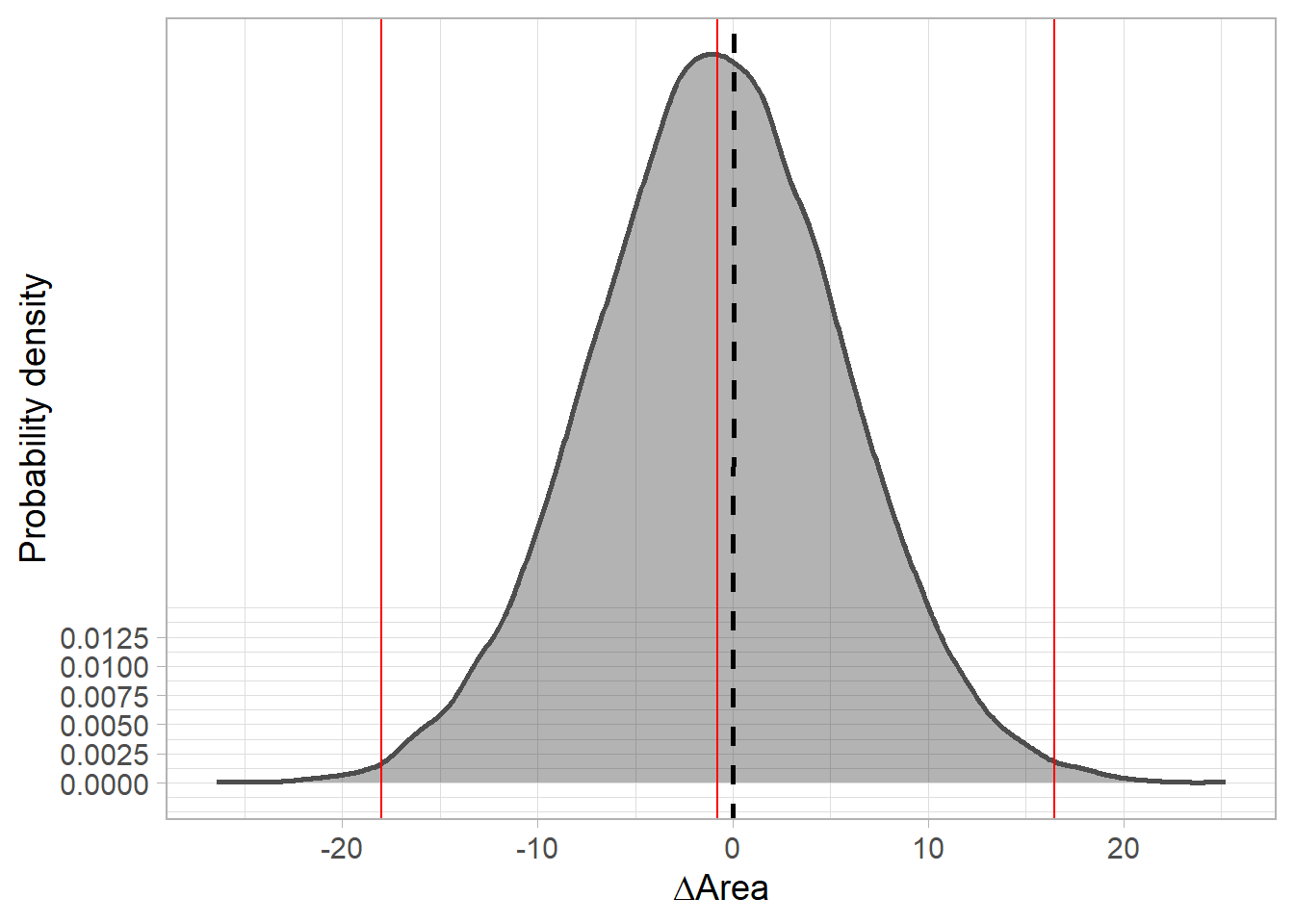

Code

ggsave(delta.A.plot, filename='docs/figs/delta_A_cthous.svg', device = 'svg', dpi=300)

posterior predictive checks

PO

Expected vs observed

Code

counts <- PO_time1_time2$count
counts.new <- fitted.model$BUGSoutput$mean$y.PO.new
lambda <- fitted.model$BUGSoutput$mean$lambda
pred.PO <- data.frame(counts, counts.new, lambda)

# fitted.model$BUGSoutput$summary['fit.PO',]
# fitted.model$BUGSoutput$summary['fit.PO.new',]

pp.PO <- ggplot(pred.PO, aes(x=counts, y=lambda), fill=NA) +
    geom_point(size=3, shape=21)  + 
    xlim(c(0, 100)) +  
    ylim(c(0, 50)) +
    labs(x='observed', y=expression(lambda), title='Presence-only') +
    geom_abline(col='red') +
    theme_bw() 

pp.PO.log10 <- ggplot(pred.PO, aes(x=counts, y=lambda), fill=NA) +
    geom_point(size=3, shape=21)  + 
    scale_x_log10(limits=c(0.01, 100)) + 
    scale_y_log10(limits=c(0.01, 100)) + 
    coord_fixed(ratio=1) + 
    labs(x='observed (log scale)', y=expression(lambda*'(log scale)'), title='log10 scale') +
    geom_abline(col='red') +
    theme_bw() 

pp.PO | pp.PO.log10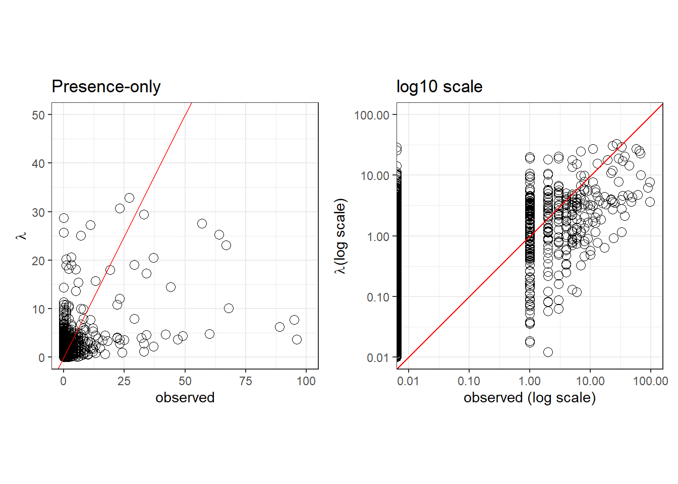

Residual Diagnostics

Code

library(DHARMa)

simulations <- fitted.model$BUGSoutput$sims.list$y.PO.new
pred <- apply(fitted.model$BUGSoutput$sims.list$lambda, 2, median)
#dim(simulations)

sim <- createDHARMa(simulatedResponse = t(simulations),
                    observedResponse = PO_time1_time2$count,
                    fittedPredictedResponse = pred,
                    integerResponse = T)

plotSimulatedResiduals(sim)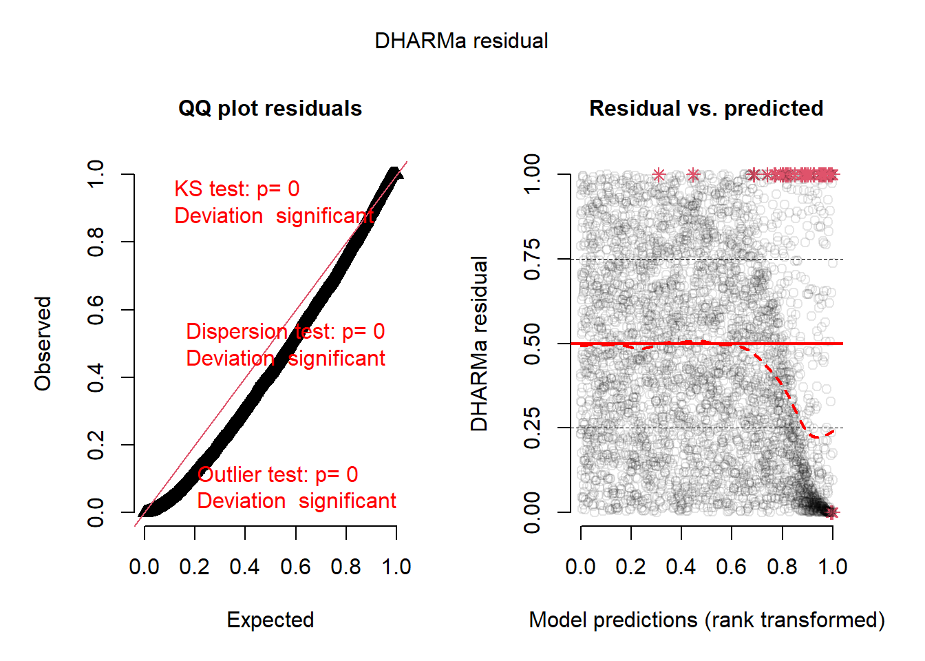

Grid-level change

Code

range_change <- as_tibble(rast2[PO_time2$pixel] - rast1[PO_time2$pixel]) %>% rename(range=time2)
numRecord_change <- as_tibble(PO_time2$count - PO_time1$count) %>% rename(numRecord=value)

grid.level.change <- bind_cols(range_change, numRecord_change) %>% 
    mutate(nonzero=ifelse(numRecord==0, '0', '>=1')) %>% 
    ggplot() +
    geom_point(aes(y=range, x=numRecord, col=nonzero), size=1) +
    geom_vline(xintercept=0, linetype=2, size=0.5) + 
    geom_hline(yintercept=0, linetype=2, size=0.5) + 
    labs(y = expression('Predicted grid-level range change (Ppred'['time2']*'-Ppred'['time1']*')'),
         x= expression('Grid-level range change in number of records (Nrecords'['time2']*'-Nrecords'['time1']*')'),
         col = 'Number of records\nper grid cell') +
    theme_bw(base_size = 14)

grid.level.change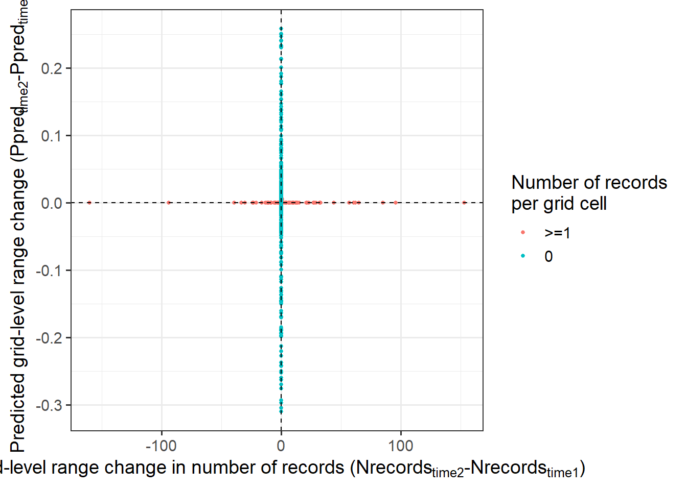

PA

Tjur R2

Code

presabs <- PA_time1_time2$presabs
psi <- fitted.model$BUGSoutput$mean$psi
pred.PA <- data.frame(presabs, psi)

r2_tjur <- round(fitted.model$BUGSoutput$mean$r2_tjur, 3)
fitted.model$BUGSoutput$summary['r2_tjur',]

          mean             sd           2.5%            25%            50% 
   0.274480158    0.005564554    0.263171394    0.270803954    0.274596102 
           75%          97.5%           Rhat          n.eff 
   0.278286565    0.285113331    1.002076443 1800.000000000

Code

pp.PA <- ggplot(pred.PA, aes(x=presabs, y=psi, col=presabs)) +
    geom_jitter(height = 0, width = .05, size=1)  +
    scale_x_continuous(breaks=seq(0,1,0.25)) + scale_colour_binned() +
    labs(x='observed', y=expression(psi), title='Presence-absence') +
    stat_summary(
        fun = mean,
        geom = "errorbar",
        aes(ymax = ..y.., ymin = ..y..),
        width = 0.2, size=2) +
    theme_bw() + theme(legend.position = 'none')+
    annotate(geom="text", x=0.5, y=0.5,
             label=paste('Tjur R-squared = ', r2_tjur))

pp.PA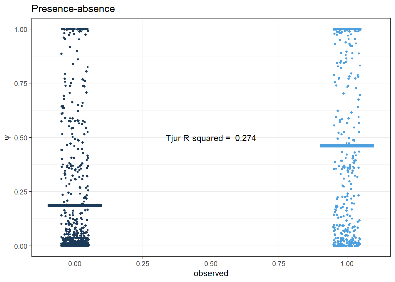

AUC

Code

auc.sens.fpr <- bind_cols(sens=fitted.model$BUGSoutput$mean$sens, 
                          fpr=fitted.model$BUGSoutput$mean$fpr) 

auc.value <- round(fitted.model$BUGSoutput$mean$auc, 3)

ggplot(auc.sens.fpr, aes(fpr, sens)) +
  geom_line() + geom_point() +
  labs(x='1 - Specificity', y='Sensitivity') +
  annotate(geom="text", x=0.5, y=0.5,
           label=paste('AUC = ', auc.value)) +
  theme_bw()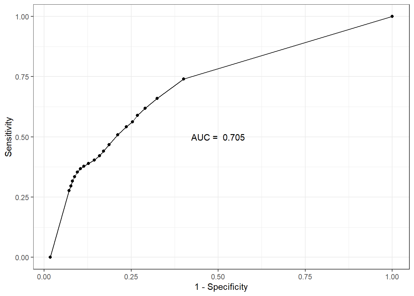

Code

fitted.model$BUGSoutput$summary['auc',]

          mean             sd           2.5%            25%            50% 
   0.705102845    0.003818685    0.697702034    0.702493244    0.705106811 
           75%          97.5%           Rhat          n.eff 
   0.707708543    0.712547143    1.001515465 3700.000000000